I love learning about computer science, lately I’ve been studying about graph theory, I even took an online course about this topic, I try to understand every concept even if it takes me longer, and I have a lemma: “If you can’t code it, you haven’t understood it”. I think this phrase is another way of saying the famous Einstein quote: “If you can't explain it simply, you don't understand it well enough”. After all, programming is explaining to a machine precisely how to proceed to solve a problem.

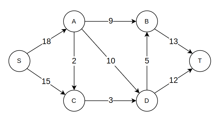
Recently I read about the Maximum Network Flow Problem, which goal is to find the maximum flow rate for a certain network. Imagine a network of pipes symbolized as a weighted graph, with a source S and a sink T (see graph below) the problem can be translated as: What is the maximum flow of water that I can put in S without the pipes breaking? There are many applications where we can use this problem (bipartite matching problem, baseball elimination, airline scheduling, and many more).

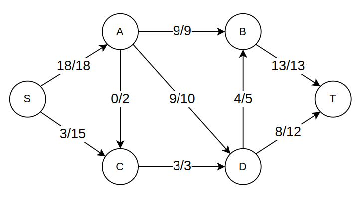
The solution for this example graph is 21, it means you can’t put in S more than 21 units of flow without “breaking” pipes. Usually there isn’t a unique graph setup to support that amount of flow, the following is one of them. As can be seen, the sum of the edge weights from S is 18 + 3 = 21.

The first approach I took to understand (implement on code) and resolve this problem was Ford–Fulkerson algorithm, I had to read many articles and watch lots of videos to achieve it. The process was a bit frustrating because there where many new concepts to learn, as for example residual graphs, augmenting paths… it was all worthy and a great experience. But then… while I was doing more research about this problem, a new mysterious concept appeared… Linear Programming (LP)! At first I thought was simply another way to solve the problem, but then I noticed the beauty and the power of this technique. With this way I was able to model and solve same problem much faster than with the previous algorithm.

But the power of linear programming is far beyond solving this particular problem. As long as you can model your problem in the way this technique needs, there is a great chance you can use it to solve it. Some examples where LP can be used are finding minimum cost perfect matching, optimal assignments, shortest path… or even solving a sudoku!.

The purpose of this article is to show this, using as example the max network problem. First I will explain the Ford-Fulkerson algorithm implementation, then I’m going to solve the same problem using Linear Programming. In order to show different LP libraries we’ll solve it using Python (pulp library), and cSharp (or-tools).

Ford-Fulkerson algorithm

I’m not going to explain in detail how this algorithm works, but I want to give some intuition about it and then compare its complexity to the LP problem modeling approach.

The input for the Ford-Fulkerson algorithm is a network capacities graph flow as shown above. Then we follow this steps:

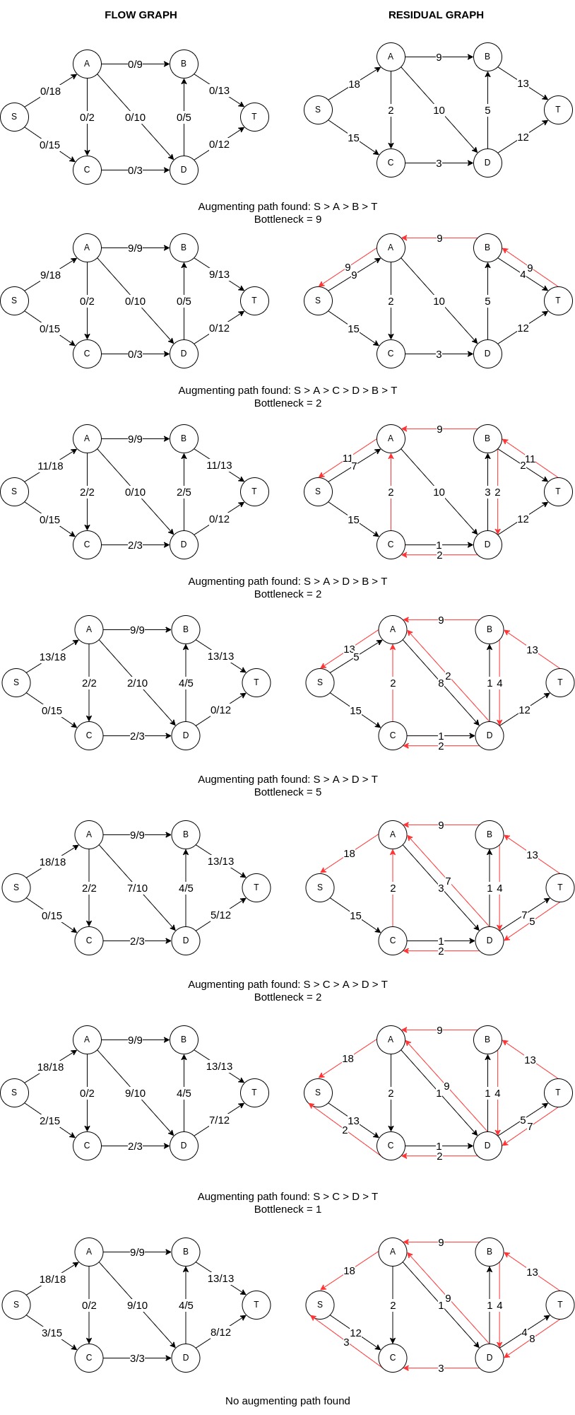
1. Initialize a flow network graph with all edge weights equal to 0. We will update this graph in each iteration. At step 0 we haven’t sent any flow, that’s the reason why all its weights are 0.
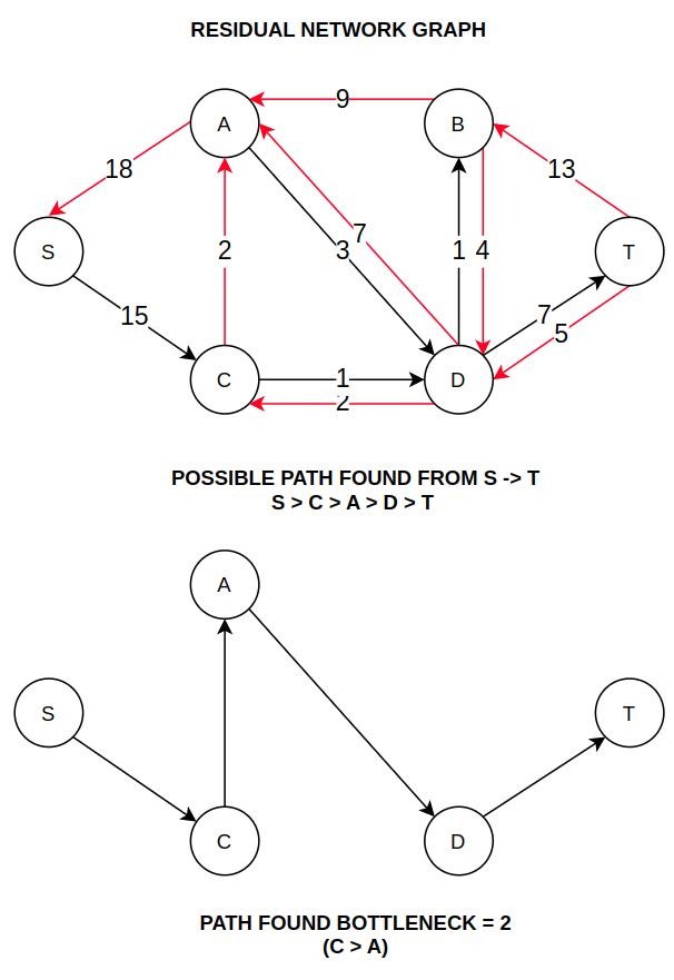
2. Initialize a residual network graph which at step 0 is a copy of the input capacities graph. This graph will be used to find possible augmenting paths. It’s important to note that once you have sent flow, you can undo it, this is represented by red lines in the figure below.
3. Find a possible path from S to T in the residual network graph. If there is a path, it means still is possible to add more flow to the network, that’s the reason why this paths are called augmenting paths.
4. Compute the bottleneck for the current augmenting path.
5. Update both flow network graph and residual network graph.
6. Go back to step 3 until there isn’t path from S to T in the residual graph.

The following images show this process for our example.

Next I show my code implementation of Ford-Fulkerson algorithm, probably can be improved in many ways, but It has all the steps mentioned before. Here I summarize briefly the code:

• getMaxFlowNetwork
  This is the main function, receives as an input the capacities graph as an adjacency matrix and returns the maximum flow.
• findPossiblePath
  Returns a possible path from S to T, for a given residual network graph, if there is no path returns undefined. Uses DFS traversal.
• getBottleneck
  Receives as an input a possible path from S to T and the current residual network graph, then returns the bottleneck, meaning the edge with minimum weight for that given path.

• updateFlowNetwork
  Updates current flow network graph receiving as an input the augmenting path found (path and bottleneck).
• updateResidualNetwork
  Updates current residual network graph receiving as an input the updated flow network graph.

You can find this code in the following Gist.

Linear Programming introduction

In a non formal way, Linear Programming is a way to find the maximum or the minimum value of a function (cost function - which has to be linear), given a set of constraints (which also had to be linear).

Example:

• Cost Function: $$ C(x_1, x_2, x_3) = 7x_1 + 3 x_2 - x_3 $$
• Constraints: $$ x_1 ≥ 0 $$ $$ x_2 ≥ 0 $$ $$ x_3 ≥ 0 $$ $$ x_1 + 2x_2 + x_3 = 3 $$

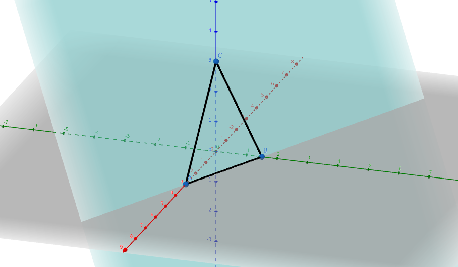
The first 3 constraints are common in all linear programming problems, they mean solution has to be in the positive octant. As we can see in the picture, last constraint is a plane. This lead us to a triangle, where one of its points will be the solution of the optimization. $$ A = (3,0,0) \implies C(A) = 7(3)+3(0)-(0) = 21 $$ $$ B = (0,1.5,0) \implies C(B) = 7(0) + 3(1.5) -(0) = 4.5 $$ $$ C = (0,0,3) \implies C(C) = 7(0) + 3(0) -(3) = -3 $$

Therefore:

• Point A lead us to the maximum of C, obtaining 21
• Point C lead us to the minimum of C, obtaining -3

Maybe you will be thinking LP isn’t a powerful tool as I said after seeing this basic example, but believe me, this tool shines because of its model simplicity. You only need a linear cost functions and constraints, but they can be far more complex than this basic example. Furthermore, you can add the constraint that variables should be integers (ILP), in fact we will use this to solve the previous Maximum Network Flow problem.

LP approach to solve Max Network Flow

In order to use LP to solve Max Network Flow we only need to model it as LP requires. As long as we can express the variables, the cost function to maximize, and the constraints (in a linear way), LP will do the job for us!

Choosing our variables

Intuitively is easy to find that our variables should be the final weights of flow for each graph edge. Then, our variables can be named as follows:

• Edge_S_A
• Edge_A_B
• Edge_A_C
• Edge_A_D
• etc…

Cost function

¿What we want to maximize? The answer is not hard to find, we want to maximize the amount of flow sent from the source (S). So, in our case:

• Cost Function = Edge_S_A + Edge_S_C

We want to find the maximum of this value.

Constraints

¿Which will be our constraints? Our intuition can lead us easily to them:

• Conservation of flow: For each node, the amount of flow received must be equal to the sent. This can be expressed using our variables as:
  • Edge_S_A = Edge_A_B + Edge_A_C + Edge_A_D
  • Edge_A_B + Edge_D_B = Edge_B_T
  • Edge_S_C + Edge_A_C = Edge_C_D
  • Edge_C_D + Edge_A_D = Edge_D_B + Edge_D_T
• Edge capacities: This is easy, each edge can’t exceed its capacity:
  • Edge_S_A ≤ 18
  • Edge_A_B ≤ 9
  • Edge_A_C ≤ 2
  • Edge_A_D ≤ 10
  • etc…

And… that’s it! This is all we need to solve the problem using LP! See how easy was to model the problem using LP compared with previous method! Of course, Ford-Fulkerson algorithm has a lot of value and it allow us to understand more about how to find a solution, but LP is like a black box that does the job for us.

LP implementation using PuLP library (Python)

PuLP is a LP Python library with a very good documentation, full of examples.

LP implementation using OR-Tools (cSharp)

Here we use another LP library called OR-Tools to solve our sample problem with c# language.

If you enjoyed this story, please click the 👏 button and share to help others find it! Feel free to leave a comment below. You can connect with me on LinkedIn, Medium, Twitter, Facebook.

Thanks for reading!