What is Monte Carlo simulation?

The term "Monte Carlo" basically associates itself with "randomness" (though, it is a city in Monaco). So, Monte Carlo simulations are actually simulations evolving randomly.

Though, this seems very counter-intuitive as to how something random can generate something useful. However, things will get clear very soon.

A close relation- Law of Large Numbers

Monte Carlo simulation is somewhat closely related to the Law of Large numbers. It basically says,

According to the law, the average of the results obtained from a large number of trials should be close to the expected value and tends to become closer to the expected value as more trials are performed

This basically means that as we go on taking more and more samples, the mean of the experiments tends to be what we expected the average to be. Obviously, we can't select an unbiased sample as it would produce a bias in our experiment. So, the best way to choose an unbiased sample is to choose randomly from a large population of samples and choose as many samples as possible.

Mathematical background

Let us have a one-dimensional function

$$f(x)$$

and a uniform distribution function

$$\rho (x)$$

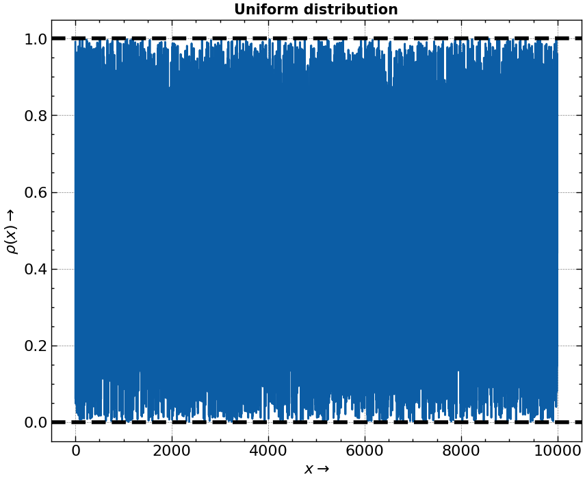
The uniform distribution function has some properties

• It is constant over its defined region.

  

• The area the distribution encloses under it is equal to 1.

  $$\int_a^b\rho(x)\;dx = 1$$

where a, b are the limits where the distribution function is defined.

$$\begin{align} Let, \; I = \int_{x = a}^{x = b} f(x) \;dx \ \ \therefore I = \int_a^b \frac{f(x) \rho(x)}{\rho(x)} \;dx ...(1)\ \ \end{align}$$

$$ \begin{align} Now, \;\; \int_a^b\rho(x) \;dx = 1. \ \ As, \rho(x) \;\; \text{is constant, so} \ \ \rho(x) \int_a^bdx = 1 \ \ \therefore \rho(x) = \frac{1}{b-a} \;\;\;...(2) \end{align} $$

$$\begin{align} From \;\; 1, \;\; I = (b-a) \int_a^b f(x) \rho(x)\;dx \ \ Now, \;\; \int_a^b f(x) \rho(x) = mean \;\; of \;\; f(x) = E(f(x)) \end{align}$$

Now, using the Law of Large Numbers and Random sampling, we can say that

$$\begin{align} E(f(x)) = \frac{1}{N}\sum_{i=1}^{i = N} f(x_i) \end{align}$$

Here are the 'i'th x elements are randomly selected and do not have any trend or pattern in their selection. So, our integral becomes

$$I = \int_a^b f(x) dx \approx (b-a) \frac{1}{N} \sum_i f(x_i)$$

Choosing the 'i'th x element randomly and continuing this for N such elements gives us our integral.

A modified form of this approach

The summation in this integral can be easily taken care of by a modified form. The basic scheme is

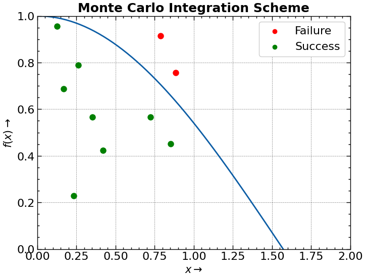
• We draw the curve on a grid

• We take random points on the grid and draw them on the graph

• If the point falls within the curve, we call it a success and if it doesn't, it is a failure.

• Let there be x successes and y failures. Then, the integral is given as

  $$I \approx \frac{x}{x+y} (b-a)$$

  Here (b-a) are the integration limits.

Code

Here, we will solve the integral

$$\int_0^{\pi/2} cos(x) \; dx = 1$$

Step 1: Import packages

Imported packages are pretty simple and very standard.

import numpy as np
import matplotlib.pyplot as plt
plt.style.use(["science", "notebook", "grid"])

Step 2: Write the logic

def decision(f, xlim:tuple, ylim:tuple, N:int) -> float:
    # Success and failure initialisation
    success, failure = 0, 0

    # Get random points for the Monte Carlo simulation
    random_x = np.random.uniform(low = xlim[0], high = xlim[1], size = N)
    random_y = np.random.uniform(low = ylim[0], high = ylim[1], size = N)

    # Logically find out about the boundaries
    for x, y in zip(random_x, random_y):
        if (y <= f(x)):
            success += 1 # success increases
        else:
            failure += 1 # Failure increases
    integral = success/(success + failure) * (xlim[1] - xlim[0]) # final ans
    return success, failure, integral

Step 3: Test our function

xlim, ylim = (0, np.pi/2), (0, 1)
N = 100
f = np.cos

final_ans = np.zeros(N) # Initialise solution array

for epoch in range(N):
    succesess, failures, final_integral = decision(f = f, xlim=xlim, ylim=ylim, N= epoch)
    final_ans[epoch] = final_integral # append final answer to array

Step 5: Visualize everything

plt.figure(figsize = (12, 8))
plt.axhline(y = 1, color = "red", linewidth = 3)
plt.ylabel("Integral", fontsize = 15, fontweight = "bold")
plt.xlabel("Iterations", fontsize = 15, fontweight = "bold")
plt.title("Monte carlo Integration", fontsize = 20, fontweight = "bold")
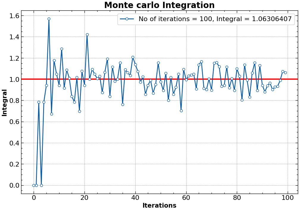
plt.plot(final_ans, "o-", markerfacecolor = "w", label = "No of iterations = 100, Integral = 1.06306407")
plt.legend()

As we see, after just 100 iterations, out integral almost converges to 1. The rate at which our integral converges is actually related to the spacing in our grid.

Obviously, in this demonstration, I have taken (b-a) to be equal to

$$\frac{\pi}{2}$$