Newton Raphson Method

Overview

In numerical analysis, finding the roots of a function is a common and essential task. The Newton-Raphson method is a widely used numerical technique for finding the root of a real-valued function. It is an iterative method that refines an initial guess to approximate the root with increasing accuracy. The method relies on approximating the function by its tangent line and iteratively updating the guess based on the intersection of the tangent line with the x-axis. By repeating this process, the method converges toward a more accurate root estimate.

How Newton Raphson Works

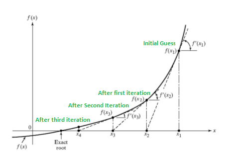
The Newton-Raphson method involves drawing a tangent line to the function f(x) at a specific point x1. The intersection of this tangent line with the x-axis provides a better estimate of the root compared to x1. This new estimate is called x2. By evaluating f(x2) and repeating the process, drawing a tangent line at x2, we refine our estimate further. This iterative approach converges towards the root of the function by successively updating the estimate using tangent lines.

The Formula

Algorithm

Here's a shorter version of the algorithm for the Newton-Raphson method:

1. Choose an initial guess for the root, x0.

2. Evaluate the function value at x0, f(x0).

3. Calculate the derivative of the function at x0, f'(x0).

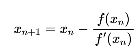
4. Compute the next approximation for the root using the formula: x1 = x0 - f(x0) / f'(x0).

5. Repeat steps 2-4 until the desired accuracy is achieved or a maximum number of iterations is reached.

The algorithm iteratively updates the guess for the root based on the function values and derivatives, aiming to converge towards the actual root. It stops when the desired accuracy is attained or the maximum number of iterations is exceeded. The final approximation, x1, is considered the estimated root of the function.

Implementation in Cpp

#include<bits/stdc++.h>
using namespace std;
vector<int>coefficients;
double f(double x){ // function for evaluating f(x)
    double result =0;
    int degree = coefficients.size()-1;
    for(int i=0;i<=degree;i++){
        result +=coefficients[i]*pow(x,degree - i);
    }
    return result;
}

double df(double x){  //function for evaluating derivative of f(x)
    double result = 0;
    int degree = coefficients.size()-1;
    for(int i=0;i<degree;i++){
        result +=coefficients[i]*pow(x,degree-i)*(degree-i);
    }
    return result;
}
int main()
{
    cout<<"Input highest power: "<<endl; 
    //This is the highest degree of the polynomial
    int n;
    cin>>n;
    coefficients = vector<int>(n+1);
    cout<<"Input coefficients: "<<endl;
    for(int i=0;i<=n;i++){
        //Input the coefficients of the polynomial
        cin>>coefficients[i]; 
    }
    cout<<"Input initial guess and tolerance: "<<endl;
    double x1,root,e; 
    //x1 is the initial guesses and e is the tolerance 
    cin>>x1>>e;
    root = x1;
    while(abs(f(root))>e)
    {
        root = x1 - f(x1)/df(x1); //Newton Raphson formula
        x1 = root; //updating x1 to the new root
    }
    cout<<"Root is: "<<root<<endl;
}

Explanation of the code

• The f(double x) function calculates the value of the equation

• The df(double x) function calculate the value of derivatives of the equation

• We have to input all of the coefficients of the calculated equation

• We also have to input the initial guesses and the tolerence

• The iterative process will continue until the value of f(x) is less than the tolerance.

Input Output of the Program

Input Highest Power :

3

Input coefficients:

1 0 -1 1

Input initial guess and tolerance:

1 0.001

Root is: 1.32482

Advantages

• Rapid convergence to the root, especially with a close initial guess.

• High precision and accuracy in root estimation.

• Efficient for well-behaved functions with smooth derivatives.

• Versatile and applicable to various types of functions and equations.

Disadvantages

• Sensitivity to the initial guess, requiring a good approximation of the root.

• Challenges with multiple roots in close proximity, lead to potential convergence issues.

• Dependency on derivative information, which may be difficult to obtain in some cases.

• Vulnerability to divergence when dealing with oscillatory or discontinuous functions.

You can also check

Horners Method For Polynomial Evaluation