Improving the Performance of Machine Learning Models - Part 1
 Yusuf Olaniyi
Introduction

"The artist who aims at perfection in everything achieves it in nothing" -
Eugene Delcroix
In pursuit of perfection, the French artist - Eugene Delcroix once said "The artist who aims at perfection in everything achieves it in nothing". The quote is not only applicable in art but in various activities ranging from cooking to drawing and this reminds me of the time I added excessive salt to my food in the quest for getting a perfect taste - you can guess what happened 😆. Like myself, at every level in the career of a data scientist or machine learning engineer, in the quest to build a perfect machine learning model, they sometimes hurt the model. Therefore, I will be sharing some tips on how to optimize the performance of a machine-learning model in this write-up.
Bias Vs Variance in Machine Learning

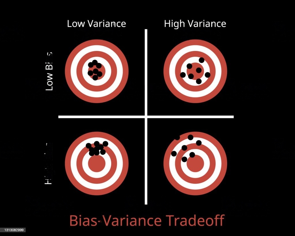
When assessing the performance of a machine learning model, two key criteria come into play: bias and variance.
Bias refers to a tendency or inclination towards something. In the context of a machine learning model, it reflects the model's ability to accurately capture the underlying patterns and relationships in the data. Imagine a chef who prepares an international dish but adds an excessive amount of sauce based on their hometown's cooking style. This bias towards a particular flavor profile may limit the enjoyment of the dish by people from different regions. Similarly, a model with high bias may struggle to generalize well beyond the specific patterns it has learned, resulting in limited performance across different data samples.
On the other hand, variance refers to the discrepancy between what is expected and what is observed. Going back to the chef's scenario, if some members of the audience can eat the food while others cannot, it highlights a variance between the expected number of people enjoying the meal and the actual number. In machine learning, variance pertains to the model's sensitivity to fluctuations in the training data. A model with high variance may overfit the training data, performing well on seen examples but struggling to generalize to new, unseen data.
Train/Dev/Test Data
To evaluate bias and variance, we typically analyze the model's performance across different datasets which include:
Training data: This dataset is used to train the model and represents the largest portion of the available data. It is like the chef's familiar region where they have honed their culinary skills.
Development data: Also known as validation or holdout data, this dataset is used to assess the model's performance during the training process. It acts as a representative sample for evaluating how well the model is learning without being biased toward the training data.
Test data: This dataset is used as a final evaluation before deploying the model to the public. It should resemble the development data and provide a realistic assessment of the model's generalization capabilities.
Data scientists strive to strike a balance between bias and variance in their models. High bias can lead to underfitting, where the model fails to capture important patterns, while high variance can result in overfitting, where the model is excessively sensitive to noise in the training data. Achieving an optimal trade-off between bias and variance is crucial for building robust and reliable machine-learning models.
| Model 1 | Model 2 | Model 3 | Model 4 | |
| Training Set | 1% | 15% | 15% | 0.4% |
| Development Set | 13% | 16% | 30% | 1.1% |
| Judgment | Low Bias and High Variance | High Bias and Low Variance | High Bias and High Variance | Low bias and Low Variance |
Considering the table above and assuming the best human performance will have an error of 0.3%. To simply understand what bias and variance mean in machine learning, bias is a measure of how far the model performance on the training set is from the best human performance while variance is a measure of how far the performance of the model on the training set and the development/test set(i.e a data that was not part of the training data).
Ideally, we strive for an algorithm that balances bias and variance. However, there are trade-offs depending on the context and resources available. Achieving the right balance involves considering the problem, data, and deployment requirements.
Generally, here are some of the common tips used when training a deep learning algorithm that has the issue of high bias and/or high variance.
High Bias | High Variance |
Train a bigger network | Get more generalized training data. |
Train the network longer | Regularization to reduce overfitting. |
Try other neural network architecture | Try other neural network architecture |
Types of Regularization Techniques
Regularization is a widely used technique to address the issue of overfitting or high variance in machine learning algorithms. It involves modifying the cost function during backpropagation by adding a regularization term. There are two primary types of regularization techniques:
L1 Regularization (Lasso Regularization): This technique adds the absolute value of the weights multiplied by a regularization parameter to the cost function. It encourages sparsity in the model by shrinking less important features' weights to zero. L1 regularization can help with feature selection and reduce model complexity.
L2 Regularization (Ridge Regularization): This technique adds the squared magnitude of the weights multiplied by a regularization parameter to the cost function. It encourages smaller weights for all features but does not lead to sparsity. L2 regularization helps in preventing large weight values and can improve generalization performance.
By incorporating regularization techniques, we can control the complexity of the model and prevent it from overfitting the training data. The choice between L1 and L2 regularization depends on the specific problem and the desired characteristics of the model.
Dropout
Dropout is a regularization technique that involves randomly deactivating a portion of nodes during the training phase. By doing so, the network becomes less reliant on specific features and learns more robust representations.
In summary, dropout helps prevent overreliance of the model on specific features by randomly deactivating nodes during training. This encourages the network to learn more diverse representations and improves generalization.
It’s important to note that dropout should not be used at test time.
Here is an example of the implementation of dropout in python.
import numpy as np

def dropout(X, dropout_rate):
    mask = np.random.binomial(1, 1 - dropout_rate, size=X.shape) / (1 - dropout_rate)
    dropout_X = X * mask
    return dropout_X

# Usage example
X = np.array([[1, 2, 3], [4, 5, 6], [7, 8, 9]])
dropout_rate = 0.2
dropout_X = dropout(X, dropout_rate)

print("Original X:")
print(X)
print("Dropout X:")
print(dropout_X)
Other Regularization Methods
Data Augmentation: This involves editing the same data to get more data for example in computer vision rotating an image or cropping a part of it is a form of data augmentation and in speech recognition problem changing the intensity or frequency of the speech is a form of data augmentation. This is generally used to have more training data to reduce variance as the model will have more experience to learn from during training.

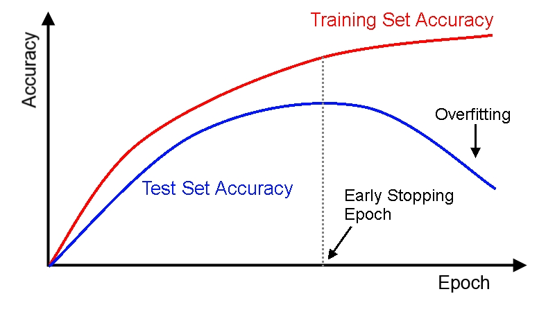
Early stopping: This is mostly employed when there are not enough resources and it involves monitoring the performance of the model to get the parameters combination that give the best performance. For example, if we have a network taking two inputs x1 and x2, with a performance shown in the plot above, we can see that the model has low bias and variance just before the dotted line so we can stop training the model and set the parameters to the parameters before the dotted line
Normalizing the inputs: This is used to increase the speed of training neural networks especially when the input data has a wide range. This is done by converting the values in the inputs from their range to a range of -1 to 1 using the normal distribution formula shown below:
x = (x - mean)/standard deviation
This would make gradient descent faster since the values computed are no longer large values. Like we have more from millions to values between 0 to 1.
Conclusion
In the quest to improve the generalisation of a machine learning model, one needs to implement any of the aforementioned regularization methods discussed based on the resources available. Another important concept which I explained in the concluding part of this series here talks about various optimisation algorithm that can be employed to enhance the convergence of machine learning algorithm while training.
Thank you for taking the time to read through this series. I appreciate your support, and I would love to hear your feedback. If you found it helpful, please consider liking, commenting, sharing, and subscribe for more insightful content. Feel free to connect with me via LinkedIn , Twitter or Email me at olaniyiyusuf2000@gmail.comfor job recommendations, projects, or potential collaborations. I’m excited to continue this learning journey with you!
Subscribe to my newsletter
Read articles from Yusuf Olaniyi directly inside your inbox. Subscribe to the newsletter, and don't miss out.
Written by
