Trajectory Stabilization using LQR

The Cart-Pole project is continuing at a steady pace. At the moment, however, I am busy working as a Robotics Intern, so the development is a little bit slower than usual. The physical system is being built by me and a friend which I will hopefully showcase in a future article. But for now, let's get into trajectory stabilization.

Rewriting code using NumPy

The old code consisted of a single CartPoleSystem class that simulated the system. On top of that, there was a CartPoleEnv class that added rendering and rewards to make it compatible with reinforcement learning. The differentiate method that was used in the explicit integration was messy and did not use NumPy and was therefore quite slow. To fix this, the code has been rewritten using NumPy and the structure has been overhauled. Now, there's a class called CartPoleDCMotorSystem that is instantiated with a Cart, DCMotor and a list of Pole objects. This system class doesn't contain any internal state and is not used for simulation. That is where the CartPoleEnv class comes in which has been overhauled to be used for simulating the system. The differentiate method has been changed to use NumPy which can be seen below. As always, the full code is available in the repository on GitHub.

import numpy as np
...

    def differentiate(self, state: np.ndarray, control: np.ndarray) -> np.ndarray:
        # x = state[0]
        d_x = state[1]
        Va = control[-1]
        thetas = state[2::2]
        d_thetas = state[3::2]

        sum1 = (self.ms*sin(thetas)*cos(thetas)).sum()
        sum2 = (self.ms*(self.ls/2)*d_thetas**2*sin(thetas)).sum()
        sum3 = ((self.u_ps*d_thetas*cos(thetas))/(self.ls/2)).sum()
        sum4 = (self.ms*cos(thetas)**2).sum()

        Ia = (Va-self.motor.Ke*d_x/self.motor.r)/self.motor.Ra
        h2 = (self.g*sum1-7/3*(1/self.motor.r**2*(self.motor.Kt*self.motor.r*Ia-self.motor.Bm*d_x)-sum2-self.cart.u_c*d_x)-sum3)
        g2 = (sum4-7/3*(self.M+self.motor.Jm/self.motor.r**2))
        dd_x = h2/g2

        dd_thetas = 3/(7*self.ls/2)*(self.g*sin(thetas)-dd_x*cos(thetas)-self.u_ps*d_thetas/(self.ms*self.ls/2))

        d_state = np.concatenate((np.array([d_x, dd_x]), np.column_stack((d_thetas, dd_thetas)).flatten()))

        return d_state
...

Linearization using SymPy

In a previous article on balancing the Cart-Pole using LQR, I omitted to show the linearization code as it's very long and not very good. I simply used the state space equations and calculated the Jacobian by hand and put that into code. The problem is that if the kinematic equations were to change, then I would have to remake those equations. Instead of doing that, there are ways of linearizing the dynamics using code.

Two different methods are either using symbolic mathematics or numerical computing. In numerical computing, the answer is numerically approximated whilst symbolic mathematics can find the precise equation and the variables can later be substituted in, giving you an answer. I chose to use symbolic mathematics using SymPy, which gives a highly precise answer, but it would later turn out that this method is quite slow which numerical computing fixes, but for now we will go forward using Sympy.

To linearize the system using SymPy, we will first have to define the state and control variables using SymPy syntax. This is done using the symbols function. In the system class, a method get_sp_vars is called in the constructor to generate the system variables. Afterward, a method called get_sp_equations is used to calculate the state space equations of the system using the same logic as the differentiate method, only using SymPy variables instead of NumPy arrays.

import sympy as sp
...

    def get_sp_vars(self):
        variables = "x dx " + " ".join([f"theta{i} d_theta{i}" for i in range(self.num_poles)]) + " Va"
        self.vars = sp.symbols(variables)
        return self.vars

    def get_sp_equations(self):
        # x = self.vars[0]
        d_x = self.vars[1]
        Va = self.vars[-1]
        thetas = self.vars[2::2]
        d_thetas = self.vars[3::2]

        f1 = d_x

        sp_sum1 = sum(m*sp.sin(theta)*sp.cos(theta) for m, theta in zip(self.ms, thetas))
        sp_sum2 = sum(m*(l/2)*d_theta**2*sp.sin(theta) for m, l, d_theta, theta in zip(self.ms, self.ls, d_thetas, thetas))
        sp_sum3 = sum(u_p*d_theta*sp.cos(theta)/(l/2) for u_p, d_theta, theta, l in zip(self.u_ps, d_thetas, thetas, self.ls))
        sp_sum4 = sum(m*sp.cos(theta)**2 for m, theta in zip(self.ms, thetas))

        h2 = (self.g*sp_sum1-7/3*(1/self.motor.r**2*(self.motor.Kt/self.motor.Ra*(Va*self.motor.r-self.motor.Ke*d_x)-self.motor.Bm*d_x)-sp_sum2-self.cart.u_c*d_x)-sp_sum3)
        g2 = (sp_sum4-7/3*(self.M+self.motor.Jm/self.motor.r**2))
        dd_x = h2/g2
        f2 = dd_x

        f_d_thetas = d_thetas       
        dd_thetas = [3/(7*l/2)*(self.g*sp.sin(theta)-dd_x*sp.cos(theta)-u_p*d_theta/(m*l/2)) for l, theta, u_p, m, d_theta in zip(self.ls, thetas, self.u_ps, self.ms, d_thetas)]
        f_dd_thetas = dd_thetas

        self.eqs = [f1, f2] + [val for pair in zip(f_d_thetas, f_dd_thetas) for val in pair] #type: ignore
        return self.eqs
...

To linearize the dynamics at an operating point, the Jacobian matrix of the dynamics needs to be calculated. This is easily done by converting the dynamic equations into a SymPy matrix and by using the jacobian function. The Jacobian is calculated in the get_sp_jacobian method. In the linearize method, the Jacobian matrix F is substituted with an operating point which results in an A and B matrix.

...

    def get_sp_jacobian(self):
        self.F = sp.Matrix(self.eqs).jacobian(self.vars)
        return self.F

    def linearize(self, state0: np.ndarray, control0: np.ndarray) -> tuple[np.ndarray, np.ndarray]:
        operating_point = {var: value for var, value in zip(self.vars, np.concatenate((state0, control0)))}
        F_evaluated = self.F.subs(operating_point)
        A = np.array(F_evaluated[:,:-1]).astype(np.float64)
        B = np.array(F_evaluated[:,-1]).astype(np.float64)
        return A, B
...

Trajectory Stabilization

In the previous article on trajectory optimization, the feedforward control is calculated using direct collocation. The feedforward signal however uses another integration method that is not explicit RK4 which is used in the simulation, which leads to integration errors. The integration errors, as well as process and measurement noise, make it impossible for the feedforward control to swing up the pendulums alone. To account for noise along the trajectory, an additional feedback LQR controller is added that tries to minimize the trajectory error. The measured state is assumed to be the full state in this setup, but this will hopefully be expanded upon later using a Kalman filter.

The LQR scheme that was developed in the last article was a discrete infinite-horizon LQR. This will however not work for trajectory stabilization. Instead, what we need now is a discrete finite-horizon LQR, which can be calculated similarly. Firstly, the system needs to be linearized along the desired trajectory that was calculated by the direct collocation algorithm. By using NumPy's vectorize, the dynamics are linearized using each row in the desired states and control as the operating points, resulting in a 3-dimensional matrix of A and B matrices for each time step in the trajectory.

dt = 0.01 # Simulation time step
end_time = 4 # Duration of the trajectory
dt_collocation = 0.05 # Time step of the collocation
N_collocation = int(end_time/dt_collocation)+1 # Number of collocation points
N = int(end_time/dt) # Number of simulation points

# Instantiate collocation solver
direct_collocation = DirectCollocation(
    N_collocation,
    system.differentiate, 
    system.state_lower_bound.shape[0],
    system.control_lower_bound.shape[0],
    system.constraints,
    system.calculate_error,
    0.001
)

initial_state = np.array([0, 0] + [radians(180), 0]*n)
reference_state = np.array([0, 0] + [0, 0]*n)

# Find a trajectory
states, controls = direct_collocation.make_controller(end_time, initial_state, reference_state, N)

# Linearize dynamics along the trajectory
As, Bs = np.vectorize(system.linearize, signature='(n),(m)->(n,n),(n,m)')(states, controls)

To perform trajectory stabilization using LQR, one first needs to be familiar with the Riccati equations. In our case, this is the Discrete Algebraic Riccati Equation (DARE). I have split this into two equations (1.1 and 1.2), where P is the unique positive definite solution to the DARE, and K is the discrete infinite-horizon LQR gain which is used for balancing the poles.

To calculate the LQR gains along the trajectory, the infinite-horizon solution won't do. Instead, we will calculate the discrete finite-horizon gains for every A and B matrix. To do this we use the dynamic Riccati equation. The LQR gains are calculated backward in time using 1.3 and 1.4.

To implement this, the FSFB and LQR classes have been rewritten to be more flexible. The class no longer has any members and the A and B matrices are provided in the methods instead. The method calculate_finite_K_ds takes in the A and B matrices along with the Q and R matrices. It first calculates the last P and K using DARE using the last state when the system should be at an equilibrium point. The gains are later calculated backward using the dynamic Riccati equation.

import numpy as np
from scipy.signal import cont2discrete
from scipy.linalg import solve_continuous_are, solve_discrete_are

class FSFB:
    def __init__(self, dt: float):
        self.dt = dt

    def discretize(self, A: np.ndarray, B: np.ndarray, C: np.ndarray, D: np.ndarray):
        dlti = cont2discrete((A,B,C,D),self.dt)
        A_d = np.array(dlti[0])
        B_d = np.array(dlti[1])
        return A_d, B_d

class LQR(FSFB):
    # Calculates the continuous infinite-horizon LQR gain
    def calculate_K(self, A: np.ndarray, B: np.ndarray, Q: np.ndarray, R: np.ndarray) -> tuple[np.ndarray, np.ndarray]:
        P = solve_continuous_are(A, B, Q, R)
        K = np.linalg.inv(R) @ B.T @ P
        return P, K

    # Calculates the discrete infinite-horizon LQR gain
    def calculate_K_d(self, A_d: np.ndarray, B_d: np.ndarray, Q: np.ndarray, R: np.ndarray) -> tuple[np.ndarray, np.ndarray]:
        P_d = solve_discrete_are(A_d, B_d, Q, R)
        K_d = np.linalg.inv(R + B_d.T @ P_d @ B_d) @ (B_d.T @ P_d @ A_d)
        return P_d, K_d

    # Calculates the discrete finite-horizon LQR gains along a trajectory
    def calculate_finite_K_ds(self, A_ds: np.ndarray, B_ds: np.ndarray, Q: np.ndarray, R: np.ndarray) -> tuple[np.ndarray, np.ndarray]:
        P_d_last, K_d_last = self.calculate_K_d(A_ds[-1], B_ds[-1], Q, R)

        K_ds = np.zeros((A_ds.shape[0], K_d_last.shape[0], K_d_last.shape[1]))
        K_ds[-1] = K_d_last

        P_ds = np.zeros((A_ds.shape[0], P_d_last.shape[0], P_d_last.shape[1]))
        P_ds[-1] = P_d_last

        for k in range(A_ds.shape[0]-2, -1, -1):
            K_ds[k] = np.linalg.inv(R + B_ds[k].T @ P_ds[k+1] @ B_ds[k]) @ (B_ds[k].T @ P_ds[k+1] @ A_ds[k])
            P_ds[k] = A_ds[k].T @ P_ds[k+1] @ A_ds[k] - (A_ds[k].T @ P_ds[k+1] @ B_ds[k]) @ K_ds[k] + Q

        return P_ds, K_ds

    # Calculates the feedback control
    def feedback(self, K: np.ndarray, error: np.ndarray) -> np.ndarray:
        u = error @ K.T 
        return u

Result

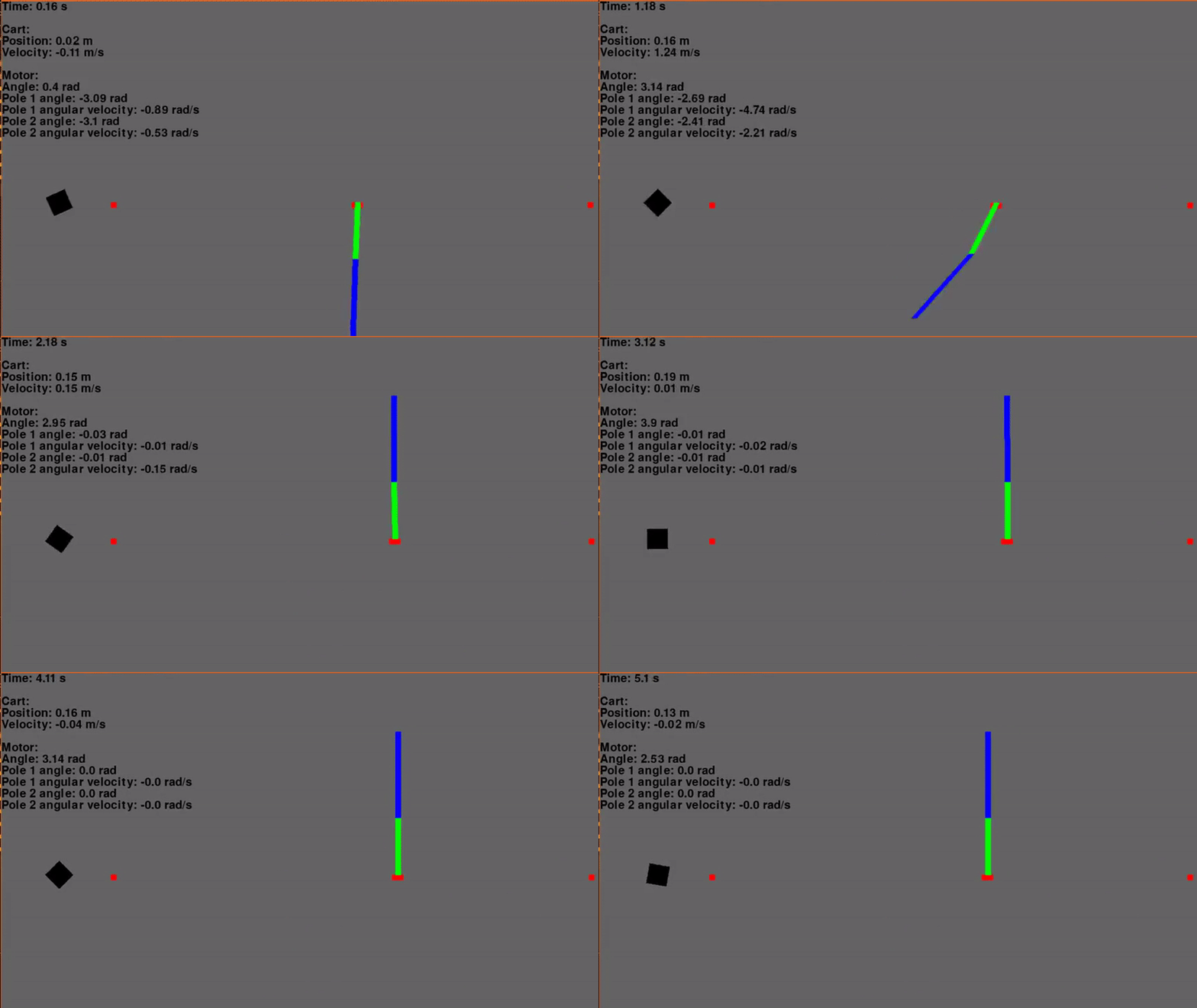
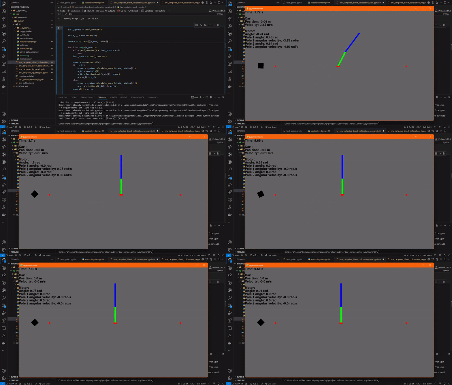
Using the aforementioned control scheme, a trajectory was generated and the feedback gains were calculated. The system was simulated with a time step of 0.01 seconds and two poles.

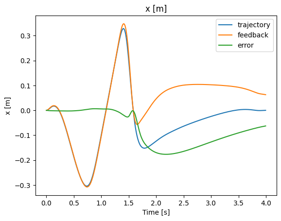
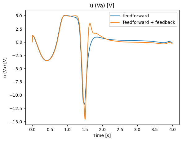
And it works very well! Granted, this is simulated without any process or measurement noise, but it is looking very promising so far! Below the position of the cart and the input voltage are graphed throughout the swing-up maneuver.

Future Development

Next up is to optimize the speed of the code as the trajectory solver and the linearization steps are pretty slow at the moment. For the trajectory solver, SciPy will be switched out to GEKKO. For the linearization, a numerical solution will hopefully be used instead.

I am currently developing the physical system with a friend and we are switching out the DC motor for a stepper motor as the balancing act needs high precision. Later on, process and measurement noise will be added to the simulation along with an observer using a Kalman filter. But that's it for now, thank you for reading!

Next part - Fast Optimization using CasADi with Opti

Previous part - Trajectory Optimization using Direct Collocation