If you've ever come across some basic use cases of machine learning, you would have probably seen that it is used for classification purposes. Let's say I have to train my machine-learning model to classify a picture as Cat or Not Cat. So we train the model on thousands and thousands of pictures of cats, usually, we use Convolutional Neural Networks (CNN) for this purpose, and eventually, after numerous epochs(iterations) of backpropagation and learning about cat pictures, it gets really good at identifying Cat pictures even if you give it a picture outside of its training set with a little bit of a side pose, standing or sitting, etc, you get the point.

Okay so let's suppose we live in a city that has a 0 plagiarism policy, where plagiarism encompasses any resource which is available on the Internet. Now, We're handed a task to draw/generate hundreds of pictures of Cats and we can't just take them off the internet. Well, we need to generate some images then, but how? My machine learning model can only classify the pictures I give it, it surely cannot generate new unseen cat pictures off of the dataset we've provided it.

Wait... Can it?

Concept Behind GANs

This is where Generative Adversarial Networks (GANs) come in. Before discussing how are they architected, let's first break down and estimate what they could be doing just off of their name. Generative might mean they must generate something, quite possibly images, what could adversarial mean?

Adversary refers to a foe, an enemy, or a rival. Generating Enemies was surely never our intention so what does it refer to? At this point let's jump into it and surely we'll realize the context of the word 'Adversary'.

GANs consist of mainly two components in their architecture namely

The "Generator" and The "Discriminator".

The Generator and Discriminator

The discriminator isn't what you think it is, a machine doesn't discriminate anyone. It can be understood as the classification model which you just trained. Let's continue with the Cat example. Our discriminator is very good at classifying cat and non-cat pictures and generally we humans give it an image off of the internet to test it.

If you think about it, it's just like how humans learn, it's how the whole education system works, you're given a syllabus, a set of topics which you need to be trained on, and you study and study for it, in and out, start to observe patterns about the topic and learn to grasp the basic concept behind it, let's think about this phase as your model training phase, then you have the Final Examination where you might have to answer certain questions which you might have never seen before, using the knowledge that you gained in your 'Training Phase'. This could be thought of as the 'Testing Phase' or testing the model's classification skills. Our Classification Model is now ready.

Let's move to the need for a 'Generator', The problem we were facing was of generating novel images, so let's build a generator model that uses prompts from the user and is based on an encoder-decoder architecture and Naive Bayes, it uses conditional probability to estimate what the output should be given the input it already has, which we have seen in the previous blog and tries to generate an image which it thinks is fit for the prompt.

Now comes the most intuitive and interesting part, at first the generator will just generate random Gaussian noise, no better than the black and white static signals that you must have seen on your CRT TVs back in the day, no matter what prompt you give it, initially the generator image will be just random noise and as you might have guessed, We would feed this image into the "Discriminator" and ask it to classify it as a 'Cat' or a 'Not Cat' image, so it would output a number between 0 and 1 , 0 meaning fake and 1 meaning real and anything between would be just probability of what is what, like 0.5 meaning could be both 50-50, it would be child's play to classify it as a Not Cat image at first. The discriminator-generator would behave something like this -:

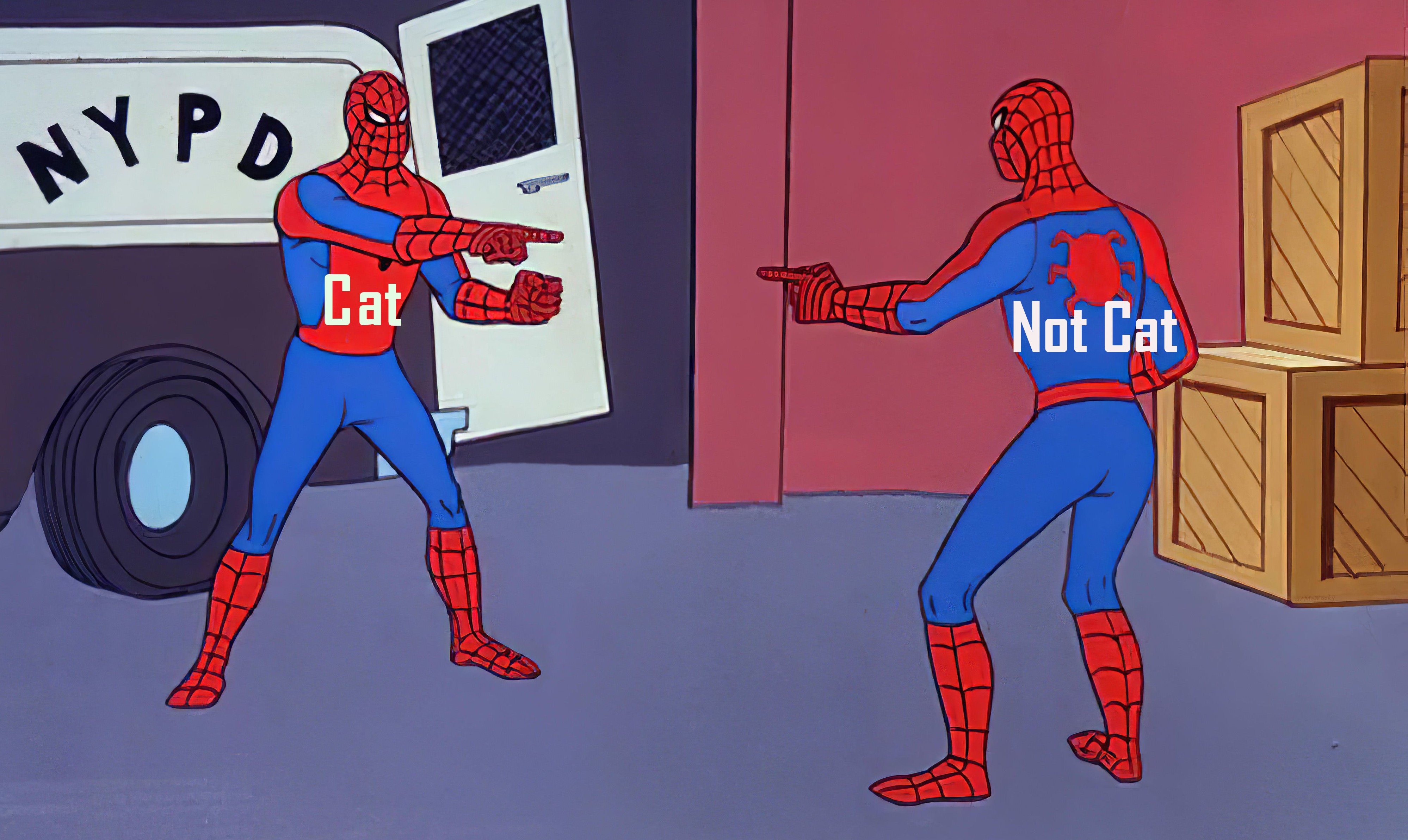
We give this "Negative" feedback to the generator, now what exactly do I mean by "Negative" feedback? For the generator, it would simply mean that it wasn't able to fool the Discriminator into classifying it as a real 'Cat' picture. At this point, you might be able to relate to why we called it an Adversarial Network.

Generator Vs Discriminator

Let's understand it better and build more intuition as to how it would help us to generate actual images that resemble the pictures we see on the internet.

From here onwards, we will treat the 'Discriminator' and the 'Generator' as Opponents, Rivals, or Adversaries, whatever floats your boat, Both of them are just submodels of our image generation model.

Treat this as a competitive game, both the submodels/rivals are pitted against each other, the Generator tries to fool the discriminator into classifying the image which it is producing as a real 'Cat' picture, on the other hand, the discriminator is trying to tell the fake from the real 'Cat' picture apart. So two models which are really bad at what they do are improving each other bit by bit till they become very good at it.

You might even think of it as a game between a thief who wants to get better and better at stealing and a police officer who wants to get better and better at catching the thief, just like in the movie 'Catch Me If You Can', the con man gets better and better at performing the con and the police is getting smarter and smarter by the day to catch him.

You vs You

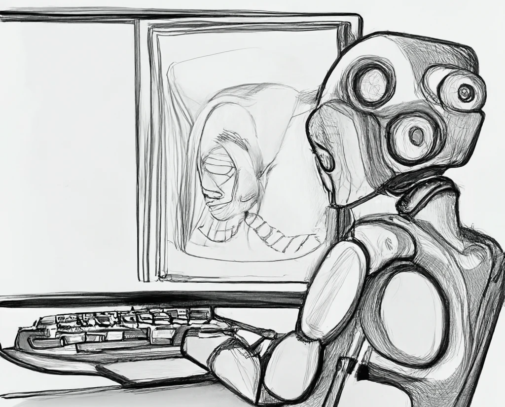
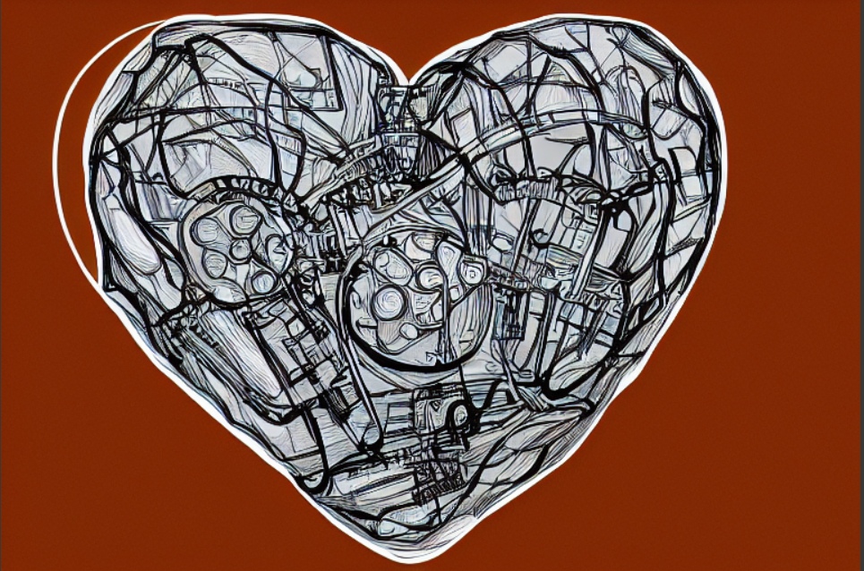
It can also be thought of as a 2 player game where the model is just playing itself. Just like when you play with your opponent you observe the mistakes that they're making, your opponent wants to exploit your mistake to make you lose, so what better way to improve your mistakes other than being your very opponent, this way you see your shortcomings and improve your game, you keep getting better at recognizing your weaknesses by playing yourself. The clever part is, It's even better because every time you play yourself, you're a better version of your previous self. So every time your game improves, your opponent also improves and if your opponent improves, it is harder to win or to fool it, so you also learn to play better and on it goes until you both become masters at the game just like a MINI-MAX game and for our use case the machine eventually gets so good, it starts producing photorealistic images of the subject. The picture shown below is AI-generated in Sketch Style.

There's one very important thing to notice here, you cannot just train the discriminator with such accuracy that it always detects the fake 'Cat' Pictures from the Real ones, why? Because if that happens the Generator would never be able to learn how to generate better fake images. So how does the generator get better at generating these images that would hopefully resemble the Real 'Cat' pictures?

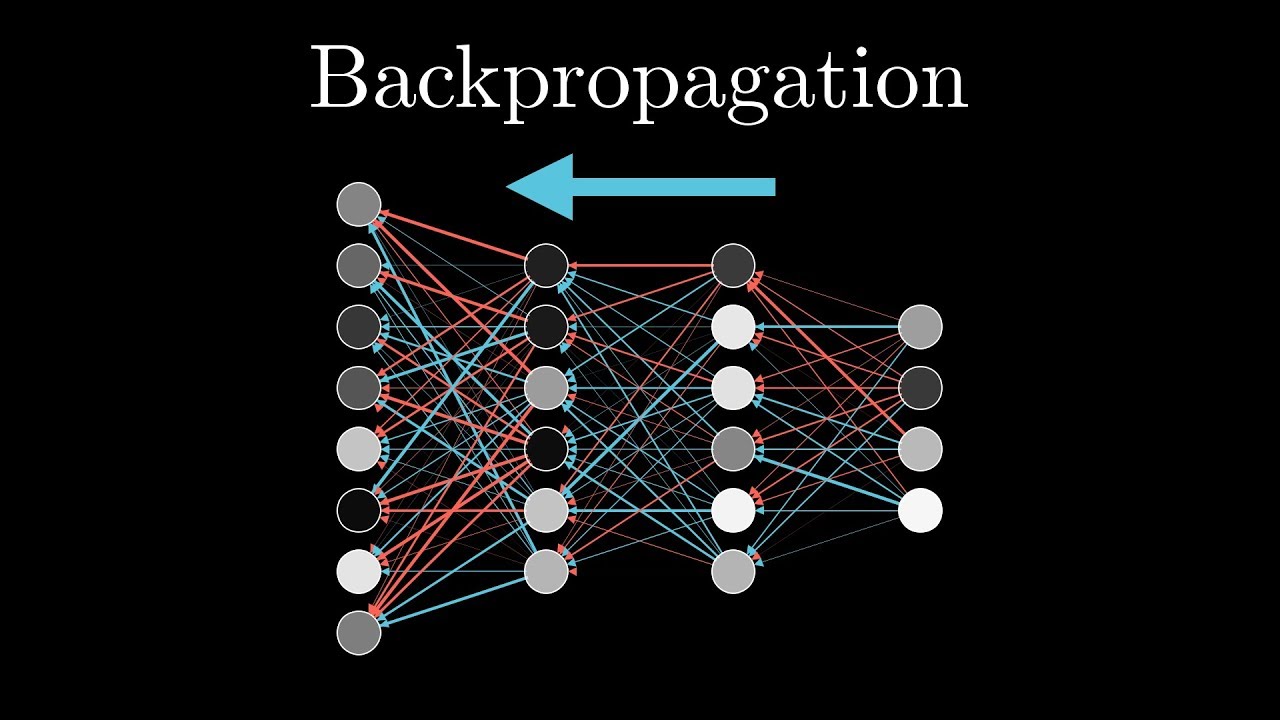
To answer that let's understand the "Machine Learning" or "Backpropagation" part of it. Whenever one of the two opponents makes any mistake, the opponent which lost that round needs to go through backpropagation and the other opponent just remains intact because it was, after all, good enough to Fool/Catch the other opponent.

Now let's answer the question. If the "Generator" loses, it uses the "Gradient of weights" from the discriminator which it needs to tweak in its model so that it can generate more compelling fake images, understand it as learning from the mistakes that it did and trying to tweak it's 'Trainable Weights' in such a manner that it could get better at fooling the discriminator.

Almost as if the discriminator is using its gradient to tell you, these weights correspond to how wrong you were so that you couldn't fool me, so learn from this, It's just like when you get your marks back, you look for the errors you made that led to you calculating the wrong answer, hence you tell your brain to learn from it and whenever you encounter it again you don't make that mistake again because you've learned from it.

By now one thing should be clear, This rivalry, this game between the Discriminator and the Generator is a Zero Sum Game. Either one has to lose every round and whoever loses learns to get better.

The contrast between both the sub-models is, both the models have exactly opposite natures. A positive feedback for the generator is a negative feedback for the discriminator and vice versa, both the sub-models also have exactly opposite gradients. Now what do I mean by this gradient?

Let's think of it as the error gap between the classification of "Real" and "Fake" Cat pictures. The Generator wants to go 'Up' in the gradient space because its positive feedback corresponds to fooling its opponent, hence it wants the discriminator to be wrong and produce erroneous results, increasing the error and hence climbing up the gradient, which means it's getting better at its task.

For the discriminator every time it catches the fake 'Cat' picture, it strives to go 'Down' the gradient space, as it's reducing the 'Loss' as we refer to, in ML, it is minimizing the loss function by getting better and better at classifying the 'Cat' pictures correctly.

Naturally, you want minimal error in detecting the pictures so 'Down' goes the discriminator, and the higher the error rate, the more times it has fooled the discriminator and we want it to be so good that it could fool it always, so 'Up' goes the Generator's gradient.

Training the Discriminator

Let's continue where we left off, the discriminator and the generator both need to be bad at doing what they do initially, now we cannot just start training both of them because the discriminator model won't have any idea what to do then.

So we first train our discriminator model on some samples of 'Real' Cat pictures and when it starts to recognize them, we slowly sample some obviously 'Fake' pictures which are not 'Cat'. Just so it can tell apart obvious 'Not Cat/Fake' pictures from 'Cat/Real' pictures. When the discriminator is trained and can do some very basic classification that is when we put both the sub-models against each other.

Training the Generator

Now the generator is given some random noise vectors which don't mean anything, these vectors are a part of what we call the 'Latent Space'. This latent space could be N-Dimensional too, now if you've read the previous blog you must know that each dimension means something to the machine, each dimension represents something about the 'Cat' picture that only the machine can comprehend and that is the reason it can generate pictures by itself, because eventually when it gets good, it actually has 'Learned' something about the 'Cat' pictures, be it their colour, the fur, the facesize, the tail, the eyes and N number of things stored in such a way in the latent space that they lie close to each other, the learnings from the N-dimensional Vectors in the latent space can also be thought of as embeddings corresponding to images.

The intuition behind the relationship between Discriminator and Generator

Now initially the generator has absolutely nothing, no learning/idea of anything at all, those vectors mean nothing, just random points in the latent space. We discussed that in the beginning the generator would produce noisy images and the discriminator because it is pre-trained a 'little bit' would be able to distinguish, now each round generator will learn to form images by incorporating the 'gradients' from the discriminator which are weighted such that they 'point towards' the label of 'Cats' and this is how it starts generating images close to the label that the discriminator has been trained on, in this case, 'Cat' pictures.

Adversaries compete to strive for perfection

Now after a certain number of victories for the discriminator, the generator would learn enough such that it can produce images that would fool the discriminator, now's the time for the discriminator to refer to the image corpora it's trained on and learn how to detect real cat pictures better.

After it learns, The generator would start to lose, then it'll learn from the discriminator again how to produce images which have a good chance of fooling it and get better and start fooling it again, and on and on, both the opponents making each other better and better and theoretically there would come a point where the Generator would get so good at generating 'Cat' pictures that the discriminator would always output 0.5 , meaning it doesn't know if the picture's fake or real, could be either it doesn't know. The Discriminator would more or less be like -:

And after this point, we don't need the discriminator because we have our extraordinary 'Cat' picture generator ready to give us tons of novel images of 'Cats'.

The generator would have learned so much about the underlying structure of how 'Cat' pictures are perceived by humans that we could even generate scenarios around cats to fit in and the generator would be able to tweak itself to generate such images by pointing to the right combination of dimensions and vector weights.

After Coming so far, let's see how well has the model done, I have generated some Cat pictures, and I will attach the prompt and the image generated with it-

AI-Generated pictures

Prompt -

"Blue eyes cat in Snow"

Image

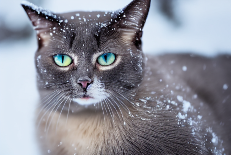
Prompt -

"Beautiful Cat Close up Sitting"

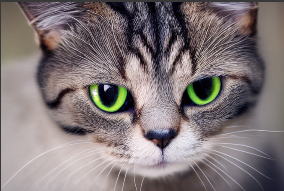
The detail and the appropriateness to the prompt are fascinating isn't it?

Juxtaposition inside the Latent Space

Now here comes the mathematically intuitive but very impressive feat achieved by GANs. We just saw that from fetching random noise vectors to creating such an N-dimensional spatial arrangement that could correspond to the different underlying features of an image, the generators do a great job of studying the subject of interest and generating novel images.

So let's train GANs on a really large dataset of Human Faces, now what happens is after we train it for long enough, the generator model eventually creates spatial regions where let's say we would find faces of men, in some other region we would find closely packed variations of women faces and when we look around in the vicinity of both these regions we could find contextual informational pieces about the image that is tweakable which could generate different features around the base face around which they lie.

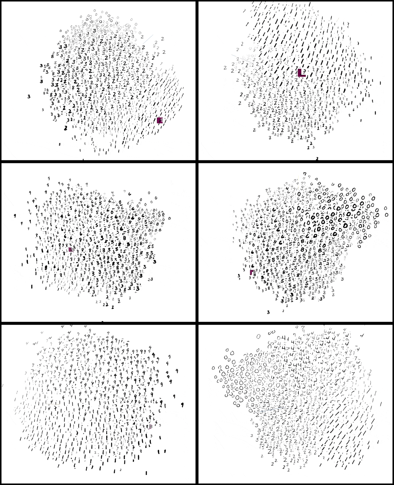
Here instead of numbers, imagine pictures and smooth variations/transitions in the pictures.

Suppose we had some wearable accessories like sunglasses, spectacles, nose rings, and such, or hair, facial hair, eye color, eyebrow style, etc.

Now what was observed was if we moved around these spatial vectors in different directions, the images would correspondingly change with the movement indicating that the machine has structured its latent space in such a way that the underlying features of the picture, actually showed up in the images just by adding, subtracting, or algebraically changing the vectors they correspond to.

This is an example of how the hair would smoothly change when moved around in the latent space.

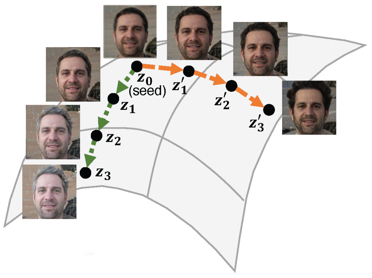
To better understand let's take an example of Lipstick, so we go near the spatial region of the generator where we have faces of Women and we skid off just a little to reach where we could see Women wearing Lipstick in the image. So now we have two regions defined namely - the faces of Women and Lipstick on the faces of Women.

Now if we take a vector that corresponds to the 'faces of Men' and ADD the vector corresponding to the 'faces of Women with Lipstick on' and then SUBTRACT the vector corresponding to just the 'faces of Women', guess what we get?

<Faces of Men> + <Faces of Women with Lipstick> - <Faces of Women> = <Faces of Men with Lipstick>

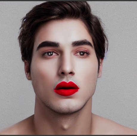
Faces of Men with Lipstick on, such simple arithmetic corresponding to such extraordinary results in the output image tells us how deeply the model learns about the underlying characteristics and features of the image to disentangle it in actual facial features.

Machines have no feelings

Let's first think about it from your perspective, if you are constantly being reminded of your flaws, weaknesses, and imperfections, after a certain point you just stop trying to improve yourself and become complacent to the fact that you'll never improve no matter how much you try and most the times if you somehow do get better at your weakness, eventually there would be other things to hammer you down. So what's the point of this? The point is that machines wouldn't feel bad if you keep hammering on their mistakes until they improve and so we do exactly that. Instead of training it for parameters at which it does fairly well, we instead focus on the parameters which are weak and keep adjusting them until the model starts constantly correcting its mistakes and improves itself by learning.

For example - If we're training our model to recognize alphabets and it's mostly doing well except for a few like 'P', 'K', 'R', and 'S', so instead of training for all alphabets equally we start focusing and feeding more variations of these alphabets so that it gets the negative reinforcement required to get better at those weaknesses particularly.

In simple words, instead of giving positive reinforcement for the things it classifies correctly, we just reduce the training on those and rigorously focus on its weaknesses, hence giving it a lot of negative reinforcements where there is a need. Hence no feelings hurt and accuracy improved.

Math Behind GANs

Let's first sum up the GAN architecture using some illustrations

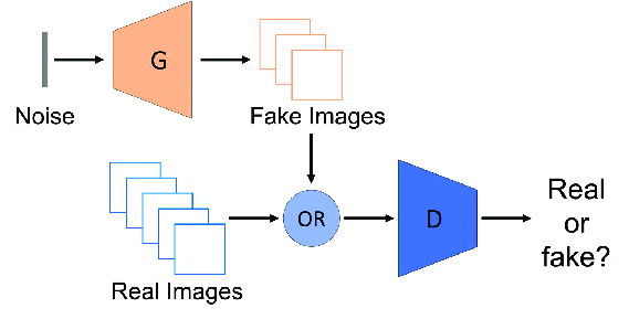
Where G refers to the Generator and D refers to the Discriminator.

Let's first look at the equation which explains GANs and we will break it down in parts to completely understand it.

$$\min_{G}\max_{D}\mathbb{E}{x\sim p{\text{data}}(x)}[\log{D(x)}] + \mathbb{E}{z\sim p{\text{z}}(z)}[1 - \log{D(G(z))}]$$

First of all, why does G want to minimize and D wants to maximize this equation?

Go back to the part where we discussed the contrasting nature of the Discriminator and the Generator. One wants to minimize the value function and the other wants to maximize it. Let's see why?

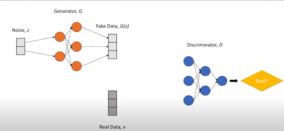
Discriminator for Real Data

Here, D(x)is the probability that the input 'x' is from the Real Data.

Now we know that x is the real data, so we just need to make sure that the discriminator should always try to maximize the term by having D(x) because that is the function giving us the confidence that Discriminator understands what the actual real data is by classifying the real data as "Real Data". But this is just for one data point x or let's say for just one image. We have tons of data, so we need to consider the average of all the data and then consider its confidence in detecting 'Real' as actually "Real", like a weighted mean.

It could also be understood as, Taking the averages of all the probabilities of the data points that translate into the confidence of the discriminator in classifying the real data as 'Real'.

$$\mathbb{E}{x\sim p{\text{data}}(x)}$$

E here symbolizes the Expectation which can also be translated to the 'weighted mean' just like we discussed. We multiply D(x) by the expectation of the probabilities of the real data which translates into one part of the equation, i.e.

$$\mathbb{E}{x\sim p{\text{data}}(x)}[\log{D(x)}]$$

Log just means that we are scaling the outputs to fit in such a way that minimizing and maximizing the function becomes relatively smooth.

Discriminator for Fake Data

Moving on, G(z) is just the input generated from the generator using random noise. So naturally, D(G(z)) should mean, ' The probability of the input being real if the input has been generated from our generator i.e. Fake Data '. So why are we seeing (1 - D(G(z)) ?

Let's look at it from the perspective of the discriminator, D(x) which was defined as the confidence of the discriminator in classifying actual real pictures as 'Real', meaning a True Positive Result. So we would of course want to maximize this term.

Meanwhile, we have the other term from the Generator, Now if D(G(z)) is the confidence of a fake input getting classified as real, then we want to minimize that term as much as possible but due to the fact that we have to maximize the whole function due to the first term getting maximized, let's convert it to an equation which would translate to getting maximized if the term D(G(z)) is getting minimized.

Hence, (1 - D(G(z)) is at its maximum when D(G(z)) is at its minimum. We again multiply it by the expectation of all the probabilities of fake data getting classified as real data, and likewise, we have the second part of the equation.

$$\mathbb{E}{z\sim p{\text{z}}(z)}$$

This whole discussion was based on the perspective of the Discriminator. So we have constructed this equation such that maximizing it, would produce better results for the discriminator, and minimizing this equation which essentially translates to doing the exact opposite would be beneficial for the Generator, hence G (min) and D (max). We have finally understood the whole equation, and putting it back together we get.

$$\min_{G}\max_{D}\mathbb{E}{x\sim p{\text{data}}(x)}[\log{D(x)}] + \mathbb{E}{z\sim p{\text{z}}(z)}[1 - \log{D(G(z))}]$$

Now let's look at the base algorithm provided in the Introductory paper on GANs.

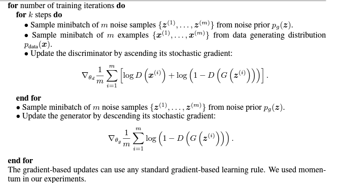
The iteration starts with training the Discriminator.

Iteration on Discriminator

In the original paper, k was taken as 1 but we can switch it up and experiment with it, we take m sample images from the real data set, and m fake sample images, provided each image has the same number of dimensions for consistency and better learning from the generator, we then feed it to the discriminator and on the basis of the results, the Value function generates its output, now we do backpropagation and we take the gradient of this Loss function with respect to the discriminator's parameters and try to train the weights of Discriminator to maximize this cost function, we just discussed the maximization part.

Iteration on Generator

We then take m fake data samples from the generator, feed them to the Discriminator, and calculate the loss function. Notice how the loss function has reduced to just one term, why?

Well because at the end we have to take the gradient of the Loss function, and D(x) would have been a constant, and the gradient of a constant term is always 0 so we do not even consider any real samples in this part of the process. Then we take the gradient of the loss function with respect to the Generator and try to minimize this cost function.

We do this for as many iterations as it takes for the GAN to start producing Good results.

Congratulations! You have understood the exoskeleton of how a GAN works and the equations and algorithms behind it.

Recent Advancements

Since the introductory paper, many types of GANs have been invented like Super Resolution GAN (SRGAN), Style GAN, and Deep Convolutional GAN (DCGAN) which excel at different problems they intend to solve. They're also used in integration with lots of novel techniques like GIRAFFE, Neural Radiance Fields(NeRFs), etc.

Recently an even better technique has emerged known as Diffusion Model, the most popular one being Stable Diffusion by Stability.ai. It has produced astounding results using de-noising and is being used heavily at the moment. Feel free to explore how it works and we might discuss it later.