Demystifying Logistic Regression

In the realm of machine learning and statistical modeling, logistic regression is a powerful algorithm used for binary classification problems. It allows us to predict the probability of an event occurring based on a set of input variables. Whether you're new to machine learning or seeking a deeper understanding of logistic regression, this comprehensive guide will equip you with the knowledge needed to apply this technique effectively. Through a series of clear explanations and real-life examples, we will build the foundation of our machine-learning concepts.

Introduction to Binary Classification

Binary classification is a fundamental problem in machine learning where the objective is to classify data instances into one of two mutually exclusive categories or classes. These classes are often referred to as the positive class (usually denoted as "1") and the negative class (usually denoted as "0"). The goal is to determine which class a given data instance belongs to based on its features or attributes.

Let's consider a real-life example: email spam detection. In this scenario, the task is to classify incoming emails as either spam or not spam. The positive class represents spam emails, and the negative class represents non-spam emails. The binary classification model analyzes various features of an email (such as sender, subject, body content, keywords, etc.) and predicts whether it is spam or not. This model helps us to focus more on important emails and also makes our inbox clean.

The key challenge in binary classification is to find a decision boundary that separates the two classes effectively. This decision boundary(usually sigmoid) is a mathematical function or rule that assigns data instances to the positive or negative class based on their feature values. Here comes the logistic regression which helps us to determine this decision boundary by modeling the relationship between the input variables and the probability of belonging to the positive class.

Sigmoid Function

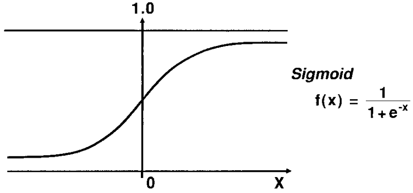
The sigmoid function, also known as the logistic function, is a crucial component of logistic regression. It plays a fundamental role in mapping the output of a linear function to a probability value between 0 and 1.

In logistic regression, the goal is to estimate the probability of an event belonging to the positive class based on a set of input variables. The linear regression part of logistic regression calculates a weighted sum of the input variables, similar to ordinary linear regression. However, instead of directly outputting this sum as the prediction, logistic regression applies the sigmoid function to transform it into a probability.

The sigmoid function is defined as follows:

f(x) = 1 / (1 + e^(-x))

Here, f(x) represents the output or probability estimate, and x represents the linear combination of input variables and their respective coefficients. The sigmoid function takes any real number as input and returns a value between 0 and 1. As x approaches positive infinity, f(x) approaches 1, indicating a high probability of belonging to the positive class. Similarly, as x approaches negative infinity, f(x) approaches 0, indicating a low probability of belonging to the positive class.

The sigmoid function has a characteristic S-shaped curve, which makes it suitable for logistic regression. By applying the sigmoid function to the linear combination of input variables, logistic regression effectively models the relationship between the inputs and the probability of the event occurring.

Equation Of Logistic Regression

In logistic regression, the linear function z is typically expressed as:

z = β0 + β1x1 + β2x2 + ... + βn*xn

Here, β0, β1, β2, ..., βn are the coefficients (also called weights) associated with the input variables x1, x2, ..., xn. The coefficients represent the impact or contribution of each input variable on the predicted probability. The sigmoid function then transforms the value of z into a probability estimate. Let's consider an example for understanding the above equation, Suppose you are a cricket fan and you want to make a bet on a fantasy cricket app upon the team which has a higher probability of winning the match. Before making the bet you will consider some conditions like pitch conditions, the current status of the team members of both teams, the previous record of both teams, etc. These conditions will be the features of our dataset and can be denoted as x1, x2, x3, ..., xn. Our logistic regression model will have the same equations as linear regression with a little change at the last, the output will have to undergo sigmoid transformation(like the Antman transformation) to be in the range of 0 to 1.

The sigmoid function's output can be interpreted as the probability of the event belonging to the positive class. For example, if the sigmoid function returns a value of 0.8 for a particular instance, it implies an estimated probability of 0.8 or 80% likelihood of that instance belonging to the positive class.

Multiclass Logistic Regression

Multiclass logistic regression extends the binary classification capability of logistic regression to handle problems with more than two classes. It allows us to predict the probability of an instance belonging to each class within a multiclass problem setting.

In binary logistic regression, we have a binary response variable (0 or 1), and the model estimates the probability of belonging to the positive class. However, in multiclass logistic regression, we deal with response variables having more than two classes. For example, classifying images into various categories, such as cats, dogs, and birds.

There are two main approaches to implementing multiclass logistic regression:

One-vs-Rest (OvR) Approach

OVR involves training multiple binary logistic regression models, where each model focuses on distinguishing one class from the rest of the classes. Suppose we have a multiclass problem with K classes. To apply the OvR approach, we create K separate logistic regression models. For each model, we designate one class as the positive class and consider the remaining K-1 classes as the negative class.

During the training phase, we train each binary logistic regression model independently. For example, let's say we have a review of a viewer about a movie on IMDB and we have to classify the review into 3 classes good, medium, bad. First, we create 3 separate logistic regression models. One model for classifying good reviews as positive and the other two reviews as negatives and respectively for each type of review. In the end, we choose the model with the highest probability and that review will belong to that particular group of reviews.

Multinomial logistic regression

It is also known as Softmax Regression and is an extension of binary logistic regression to handle multi-class classification problems directly. Instead of training multiple binary classifiers as in the one-vs-rest approach, the multinomial logistic regression algorithm trains a single model that can assign probabilities to multiple classes.

Let's consider a multi-class classification problem with k classes, similar to the one described before. In multinomial logistic regression, we introduce a weight matrix W of size (n_features, k) and a bias vector b of size (1, k), where n_features is the number of input features.

Given an input sample x, the hypothesis function for multinomial logistic regression calculates the probability that x belongs to each class i as follows:

Here, W_i and b_i represent the i-th column of weight matrix W and bias vector b, respectively. The softmax function is used to ensure that the probabilities sum up to 1.

The cost function in multinomial logistic regression is the cross-entropy loss, which measures the difference between the predicted probabilities and the true class labels. The cost function for a single training example is given by:

&space;=&space;-%5Csum_%7Bi=1%7D%5E%7Bk%7Dy_i%5Clog(p(y=i%7Cx)) align="left")

Here, y_i is the true class label, and p(y=i|x) is the predicted probability of class i given input x.

To predict the class for a new input sample x, we use the trained parameters W and b to calculate the probabilities of x belonging to each class using the hypothesis function. The class with the highest probability is then assigned as the predicted class for x.

The multinomial logistic regression algorithm allows for direct training of a model that can classify input samples into multiple classes. It is widely used in machine learning for multi-class classification tasks, where the classes are mutually exclusive.

Conclusion

Logistic regression is a widely used algorithm in various domains due to its simplicity, interpretability, and effectiveness in binary classification problems. It is used in medical diagnosis, credit risk assessment, fraud detection, sentiment analysis, quality control, image and object recognition etc. These are just a few examples of the many real-life applications of logistic regression.

It's the first thought of a machine learning engineer when comes to the classification problem. You can interpret it like Ronaldo of the classification problem.