Time-series forecasting with PyTorch and InfluxDB

Introduction

Time series data (also known as time-stamped data) refers to a collection of observations (data points) measured over time. When plotted on a graph, one of the axes for this type of data will always be time. Because time is part of every observable entity, time series data can be used in all kinds of industries, like the stock market, weather data, logs, and traces.

InfluxDB is an open-source database management system that specializes in storing time series data and helps organizations build real-time analytics and cloud applications. It’s a comprehensive platform that supports the collection, monitoring, and visualization of time series data.

In this article, you’ll learn the basics of InfluxDB, including how to set it up in the cloud, how to configure a client to communicate with it, and how to fetch data from the InfluxDB Cloud. You will also learn how this data can be used to train a model on PyTorch and make predictions. PyTorch is an open-source machine learning framework with features like scalable distributed training and optimization that accelerates workflows into production.

What Is InfluxDB

InfluxDB is a time series data platform built solely for time series data. The newest release, InfluxDB 2.0, written in Go, can be used as a cloud service known as InfluxDB Cloud and has a web interface for data processing and visualization.

InfluxDB offers features like the following:

• Support for multiple data types

• No network protocol issues during data transmission regardless of the number of fields and tags

• Ability to encode metadata along with time series data

• Nanosecond precision in time stamps (essential for scientific computing and finance)

Note: Field values refer to the data associated with the field key. This could be strings, floats, integers, or any other data type. A field value is always associated with a time stamp because InfluxDB is a time series database. A combination of field-key and field-value pairs is known as a field set. A field set is an unindexed, mandatory piece in the InfluxDB structure.

In use, InfluxDB has helped Rolls-Royce Power Systems improve the operational efficiency of its manufacturing plants by providing efficient data storage, performance monitoring in real time, identification of seasonality and trends, and prediction of maintenance needs. This has exponentially reduced expensive engine breakdowns and accelerated growth.

It has also helped Texas Instruments monitor and improve production and quality assurance. With InfluxDB, Texas Instruments was able to identify and troubleshoot inefficiencies in real time on their production line, thereby improving product standards.

Getting Started with Time Series Forecasting

Now that you know more about InfluxDB, you can set up InfluxDB and have it communicate with the Python client and pull data so that you can use that data for forecasting.

Set Up InfluxDB

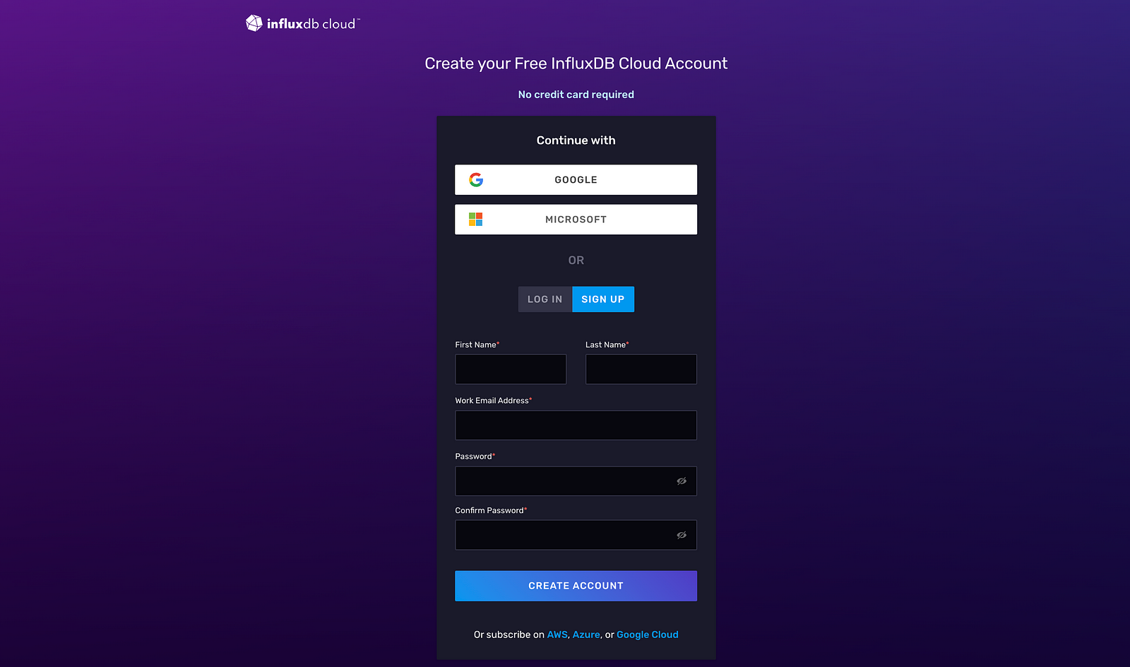
To begin, you need to set up an account with InfluxDB that can be used to integrate with other clients seamlessly. Sign up and enter the required information:

Once the account is created, specify a Provider and Region, and specify the Company Name as “NA”:

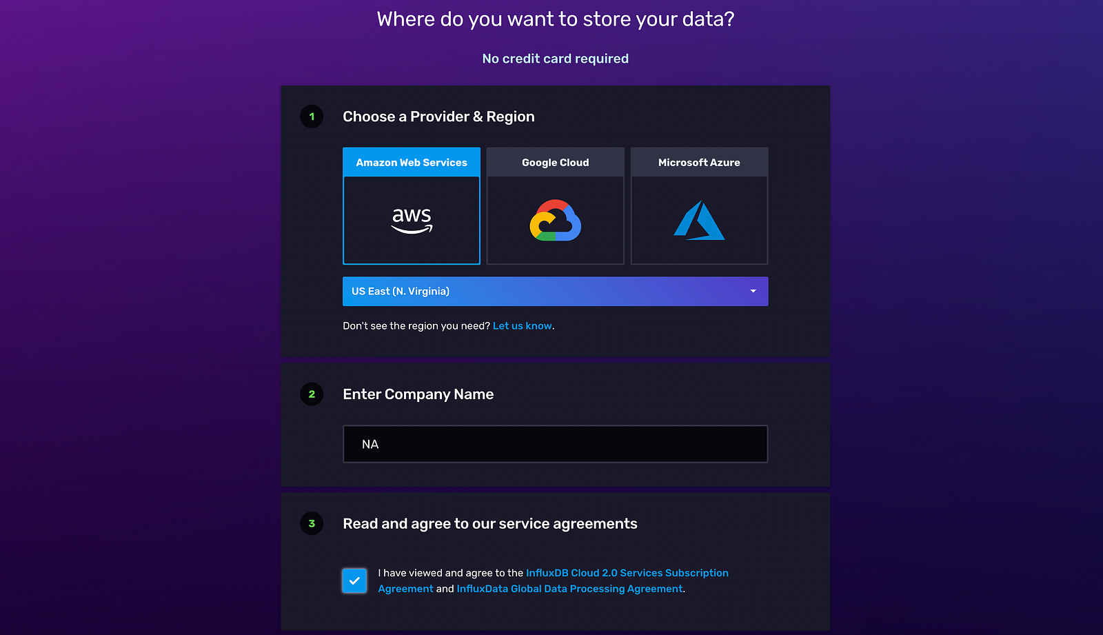
View and agree to the service subscription agreement, and select Continue in order to choose a plan:

When choosing a plan, select the Free subscription. Now, you’ve successfully created an InfluxDB account. You’ll automatically be taken to the Getting Started page of your InfluxDB dashboard. From here, you can explore how to connect to InfluxDB from different clients, push data, generate Flux queries, and visualize time series data:

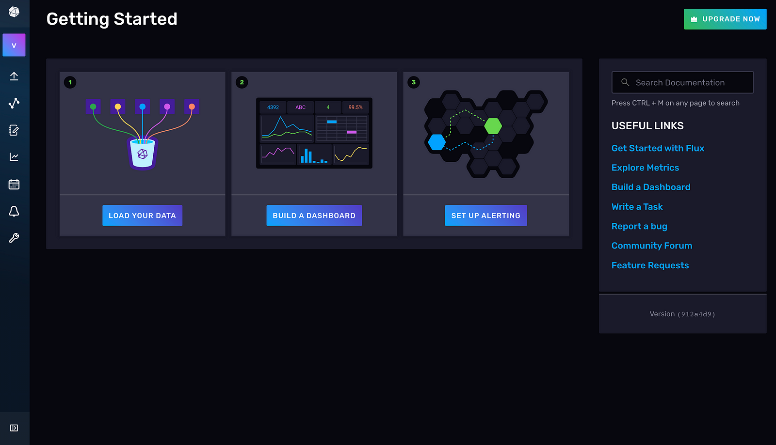
To communicate with the InfluxDB client (Python), a list of credentials needs to be specified in the Python script.

Set Up Your API Token and Bucket Name

The credentials required to communicate with the client include an API token, an organization, a bucket name, and a URL. A bucket is a unit of storage that has a retention period (that is, the time period for which data is stored in the bucket). An organization is a workspace for users.

To generate an API token, go to the API Tokens tab in the UI:

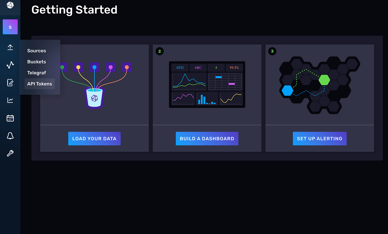
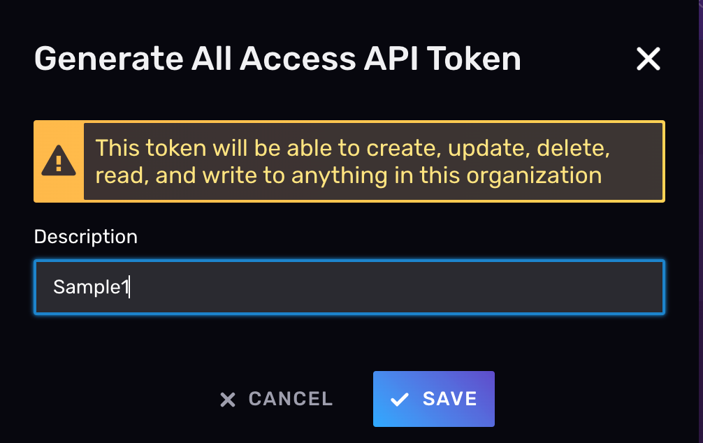
Click on GENERATE API TOKEN and select the All Access API Token:

Provide a name for the API token (for example, “Sample1”) and copy the value. Store it securely. If you lose your API token, you’ll have to create a new one because you can’t access the value of the API token later:

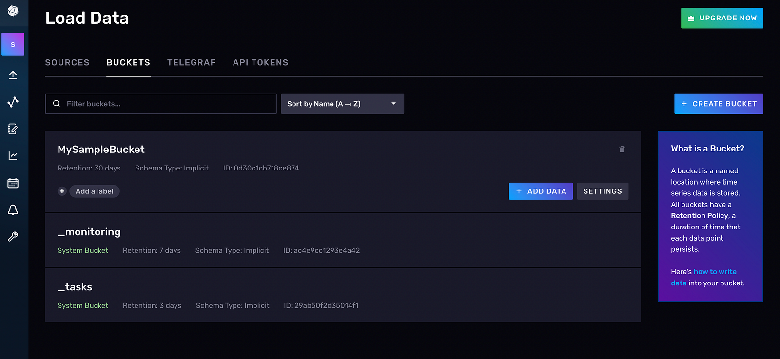
Now, you need to create a bucket by navigating to Buckets from the navigation bar on the left:

Then click on CREATE BUCKET. If you wish to rename the bucket, you can go to Settings > Rename. This isn’t recommended since you will need to update the bucket name throughout the script, and this may result in unintentional consequences, like an ApiError or ConnectionError, and the inability to connect to InfluxDB Cloud:

Install the InfluxDB Python Library

Once you have an account set up on InfluxDB Cloud, you need to install the Python client so that a communication pipeline is established between the cloud and the client.
For pip installations, use the following:

pip install influxdb-client

For macOS installations, use this:

brew install influxdb-client

You’ve now installed the necessary dependencies.

Configure the Client to Communicate with InfluxDB Cloud

After installing the client, you need to configure it to communicate with InfluxDB by specifying a list of credentials. To confirm that a connection has been established, execute a simple Flux query, and check if the data in InfluxDB matches the data you just fetched:

from influxdb import InfluxDBClient

# Fill in the below attributes after creating an account on InfluxDB Cloud
token = “YOUR_TOKEN_HERE”
org = “YOUR_EMAIL_HERE”
bucket = “YOUR_BUCKET_HERE”
# url depends on the region selected during sign up, an example is <url= “https://europe-west1-1.gcp.cloud2.influxdata.com">
url = “YOUR_URL_HERE”
client = InfluxDBClient(url=url, token=token, org=org, debug=True)
“””
Flux query execution/other source code
“””
results=[] # create an empty list
query = “””option v = {timeRangeStart: -30d, timeRangeStop: now()}
from(bucket: “myBucket”)
|> range(start: v.timeRangeStart, stop: v.timeRangeStop)
|> filter(fn: (r) => r[“_measurement”] == “stallion_data”)”””
tables = client.query_api().query(query, org=org)
for table in tables:
for record in table.records:
results.append(
[ record.get_field(),
record.get_value(),
record.get_measurement(),
]
) # append the values fetched into a list

Install PyTorch

Install PyTorch and PyTorch Forecasting since PyTorch Forecasting is built on top of PyTorch Lightning.

If you are on a Windows machine, run the following:

pip install torch -f https://download.pytorch.org/whl/torch_stable.html.

If you are on macOS, run this:

pip install pytorch-forecasting

For Conda installations, you can use the following:

conda install pytorch-forecasting pytorch -c pytorch>=1.7 -c conda-forge

Explore the Data Set

In this tutorial, you’ll use the Stallion data set present in PyTorch Forecasting. This data shows the sales of various beverages in US dollars. Your goal will be to predict the sales for the next six months, using historical sales data of 21,000 monthly records.

Stallion data contains the following data sets:

• pricesalespromotion.csv holds the price, sales, and promotion in dollars

• historicalvolume.csv contains sales data

• weather.csv has the monthly average maximum temperature

• industrysodasales.csv holds industry-level soda sales

• eventcalendar.csv holds event details (sports, carnivals, etc.)

• industry_volume.csv has the actual beer volume in the industry

• demographics.csv holds demographic details

There are several different methods you can use to load data from a client into InfluxDB, including ingesting a Pandas DataFrame, uploading a CSV file using annotations, using and consuming an InfluxDB API/write endpoint, or
using the influx write command.

In this instance, since you’re using your own data set (Stallion data from PyTorch), you need to push the data (stored as a Pandas DataFrame) to the InfluxDB Cloud first and then fetch it.

Then write a Flux script to query this data into your client environment from the InfluxDB Cloud using the following code snippet:

results = []
with InfluxDBClient(
url=”https://us-east-1-1.aws.cloud2.influxdata.com", token=token, org=org
) as client:
query = “””option v = {timeRangeStart: -30d, timeRangeStop: now()}

from(bucket: “myBucket”)
|> range(start: v.timeRangeStart, stop: v.timeRangeStop)
|> filter(fn: (r) => r[“_measurement”] == “stallion_data”)”””
tables = client.query_api().query(query, org=org)
for table in tables:
for record in table.records: # results.append(record)
results.append(
[
record.get_field(),
record.get_value(),
record.get_measurement(),
record.get_time(),
record.values.get(“agency”),
record.values.get(“sku”),
]
)

# convert the list to a dataframe
influx_df = pd.DataFrame(
results, columns=[“_field”, “_value”, “_measurement”, “time”, “agency”, “sku”]
)

Note: If you’re using the free tier, there are certain limitations that come with it. For example, you can’t go past thirty days in the time stamp of your data, and you can’t write more than a specific number of rows in InfluxDB. The priced model is an option for overcoming these limitations.

Following is an example of what your data should look like in the InfluxDB UI:

Inspect and Clean Data

One of the most important steps in any forecasting pipeline is to understand the data set, which will give you an idea of the quantity, units, and terminologies associated with the data. Then you need to clean up the data to eliminate outliers, missing values, and discrepancies. This cleaned data will be easier to process, build a model with, and make predictions.

Stallion data is relatively clean and features like time_idx (time index that is incremented by one in every step) and month (extracted from the date column) are extracted.

Note: If you’re using a different data set, data-cleaning steps will involve deleting rows that have NaNs or NaTs. You can also delete rows that have missing information or redundant rows.

Feature Engineering

One of the requirements of time series data is that it should have a column that shows the time stamp or date and time, which is an important feature for prediction purposes.

In the Stallion data set, time_idx plays that role, which is converted into the index of the dataframe. Additional features, like month and log_volume, have been added, which will contribute to improving the accuracy of forecasting.

Since you can use PyTorch Forecasting for predictions, you need to convert the data set into a “TimeSeriesDataSet”, which is a PyTorch data set, for ease of processing, analysis, modeling, and fitting the data:

training = TimeSeriesDataSet(
stallion_df[lambda x: x.time_idx <= training_cutoff],
time_idx=”time_idx”,
target=”volume”,
group_ids=[“agency”, “sku”],
min_encoder_length=max_encoder_length
// 2, # Encoder length should be long since it is in the validation set
max_encoder_length=max_encoder_length,
min_prediction_length=1,
max_prediction_length=max_prediction_length,
static_categoricals=[“agency”, “sku”],
static_reals=[“avg_population_2017”, “avg_yearly_household_income_2017”],
time_varying_known_categoricals=[“special_days”, “month”],
variable_groups={
“special_days”: special_days
}, # a group of categorical variables is treated as a single variable
time_varying_known_reals=[“time_idx”, “price_regular”, “discount_in_percent”],
time_varying_unknown_categoricals=[],
time_varying_unknown_reals=[
“volume”,
“log_volume”,
“industry_volume”,
“soda_volume”,
“avg_max_temp”,
“avg_volume_by_agency”,
“avg_volume_by_sku”,
],
target_normalizer=GroupNormalizer(
groups=[“agency”, “sku”], transformation=”softplus”
), # use softplus and normalize by group
add_relative_time_idx=True,
add_target_scales=True,
add_encoder_length=True,
allow_missing_timesteps=True,
)

For this data set, you use a single-step model (that is, the “TemporalFusionTransformer”), which is Google’s state-of-the-art deep learning model that forecast time series. This network has outperformed Amazon’s DeepAR by 36–69 percent in benchmarks:

tft = TemporalFusionTransformer.from_dataset(
training,
learning_rate=0.03,
hidden_size=16, # number of attention heads. Set to 4 for large datasets
attention_head_size=1,
dropout=0.1,
hidden_continuous_size=8, # set to <= hidden_size
output_size=7, # 7 quantiles by default
loss=QuantileLoss(), # reduce learning rate if no improvement is seen in the validation loss after ‘x’ epochs
reduce_on_plateau_patience=4,
)
print(f”Number of parameters in network: {tft.size()/1e3:.1f}k”)

The output is as follows:

Number of parameters in network: 29.5k

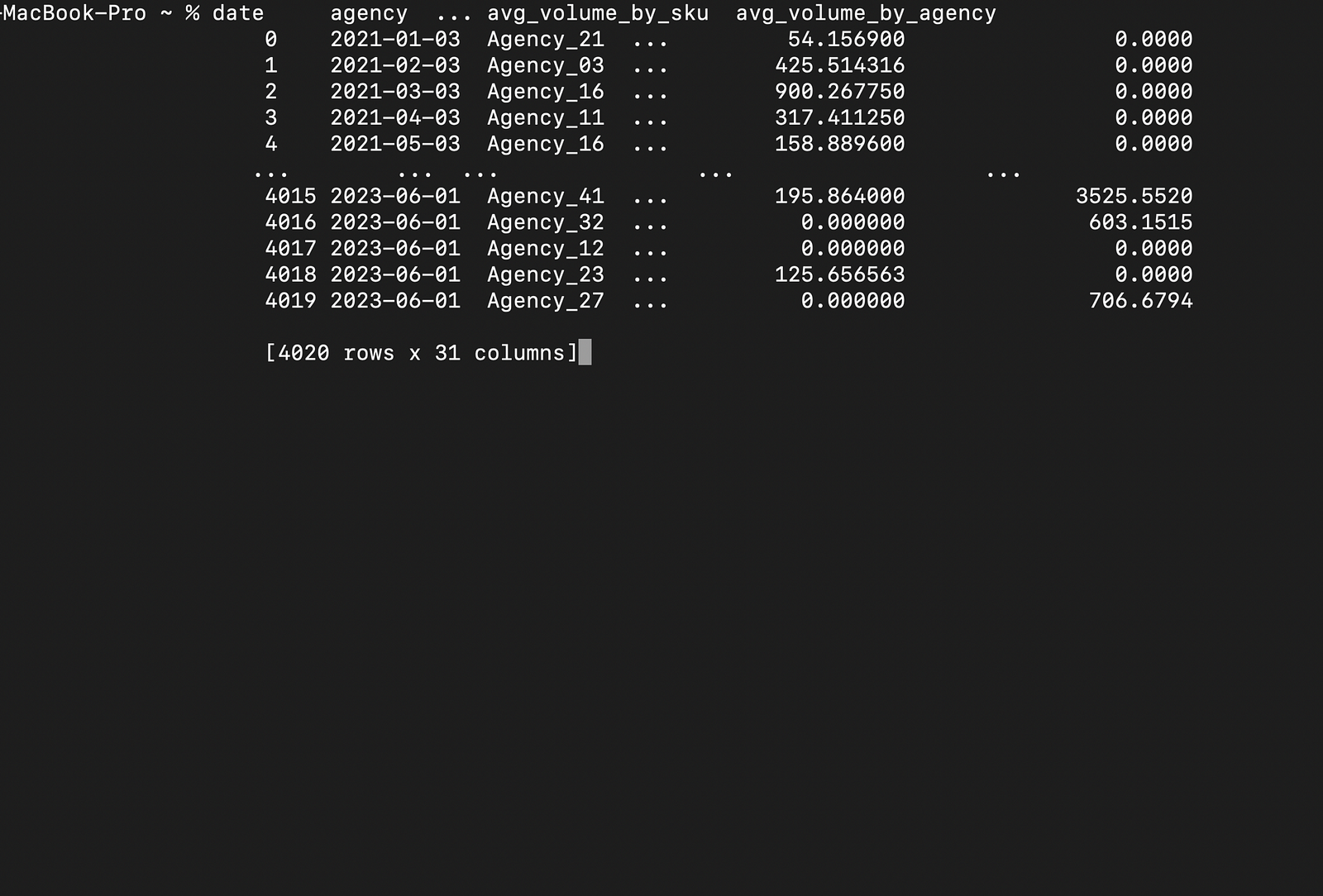
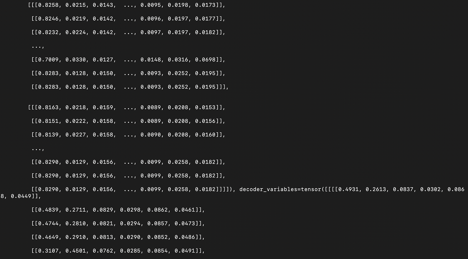
Here, you use the “TemporalFusionTransformer” to build the model and fit the Stallion data to it. Then you use “predict()” to generate predictions on new data (that is, the data for the next six months). The final output, pytorch_forecasting.utils.TupleOutputMixIn.to_network_output.<locals>.Output, shows the volume for the next six months of data.

Below is a sample output for the dataframe with the next six months of data:

And here is the prediction of the volume for the next six months:

All the code for this article can be found in this GitHub repo.

Conclusion

In this article, you learned how InfluxDB can efficiently store and process time series data. You were able to see that InfluxDB’s UI is interactive, easy to use, and can create buckets, add data, and generate Flux queries in multiple languages.

InfluxDB automatically builds Flux queries once you select the data you wish to visualize. It can build client code (that embeds the Flux query as a string), which can be executed in client IDEs.

InfluxDB also has InfluxDB OSS that can be installed and used locally.
Apart from the Python client, it can be integrated with many other clients, and you can use plug-ins like Telegraf, an open-source data collection agent that can communicate with databases, sensors, services, and third-party APIs.