Algorithms, Algorithms, Algorithms
 Olivier Hinds
Table of contents

About My Blog
I have decided to start a blog, in order to improve both my writing skills, and my ability to research topics I enjoy and share my learning experiences with the world. I have chosen to write blogs quarterly, however, I may include some special releases when I have some extra time. If you have any feedback or advice, please reach out via email. Enjoy!
The JPEG Algorithm
JPEG (Joint Photographic Experts Group) is one of the oldest image compression standards of all time. It is a method of lossy compression that takes an image and reduces its file size by removing parts of the image that we “do not see” as well. This process takes away a lot of unnecessary information, that we would not perceive anyways. The reason I wanted to take a look at the JPEG algorithm is because of all the inner workings.

The JPEG Logo
How JPEG Works
As previously mentioned, the JPEG algorithm is very complex and has many parts. Here is a breakdown of the parts, and what they do. I will go into more detail further on.
Colour Space Transformation
Downsampling
Block Splitting
Discrete Cosine Transform
Quantisation
Entropy coding
So, what do these mean exactly?
Colour Space Transformation
As you will probably know, almost all images online are stored with the RGB colour space, meaning each pixel has a Red, Green, and Blue component. These values are from 0 --> 255, meaning they use 8 bits to store each component value. The JPEG algorithm takes advantage of human’s perception of luminance and chrominance and therefore requires the Y'CbCr colour space.
Note: There are plenty of colour spaces out there, Y'CbCr just happens to be the digital representation of YUV (Analogue; often used in video formats). There are other, potentially better colour spaces like YCoCg which are faster computationally and lossless (in conversion).
Find more information about YCoCg on the wiki Here
After converting our original image into Y'CbCr, we now have 3 values called luma (Luminance), and two chroma (Chrominance) values.
Y'CbCr allows for compression without much of an effect on the quality we can perceive.
Downsampling
In the human eye, we have 2 different types of light receptors. Rods and cones. These are distributed as follows:
| Name | Quantity | Function |
| Rods | 120 Million | Perceive light well, do not perceive colour. |
| Cones | 5 Million | Capable of perceiving colour, at higher light levels. |
Ahh… We have a lot more Rod cells then cone cells. This means that humans perceive / respond to light more than they do colour.
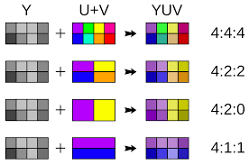
The JPEG algorithm exploits this by keeping theY' component of the image as true to the original, and performing a “chroma subsample” or downsample on the other two components; Cb, and Cr.
This essentially reduces the “samples” in the image, by making larger pixels with an interpolated colour value from 4 surrounding particles

Chroma Subsampling in action, with compression ratios on the right.
Block Splitting
Next, we must split the image into 8×8 blocks (The smallest block of pixels in the image). This is called the Minimum Coded Unit (or MCU).
Potential errors:
- Our image could potentially not be in an aspect ratio divisible by 8 (say 20×20), and then we would have to turn the image into a 24×24 image by filling in the pixels with black or some other form of dummy data.
We perform block splitting to make our next step easier.
Discrete Cosine Transform
Here is where the maths is… We need to convert this image into what's known as a frequency domain.
Essentially, this is representing the image by showing the different frequencies that make up the image.
The specific type of frequency domain conversion used on a JPEG image is a “normalised, two-dimensional type II DCT” (DCT-II), meaning that we can compress the image effectively, whilst preserving the image quality as much as possible.
The DCT generates an array of coefficients that condense the image or “concentrate” the colour signals into a more compact form.
Here is an example of an 8×8 MCU from an image:
$$\begin{bmatrix} 57 & 242 & 81 & 104 & 141 & 68 & 195 & 160 \\ 193 & 160 & 17 & 73 & 25 & 28 & 22 & 212 \\ 131 & 9 & 222 & 218 & 38 & 165 & 136 & 245 \\ 89 & 105 & 136 & 146 & 97 & 208 & 20 & 185 \\ 190 & 185 & 82 & 85 & 135 & 132 & 5 & 203 \\ 45 & 56 & 199 & 121 & 37 & 121 & 222 & 170 \\ 103 & 25 & 56 & 223 & 48 & 185 & 200 & 54 \\ 230 & 233 & 228 & 34 & 59 & 179 & 216 & 182 \\ \end{bmatrix}$$
The formula for a DCT-II transform is given below:
$$C(u, v) = (\frac{2}{N}) cos(\frac{(2x+1)u\pi}{2N}) cos(\frac{(2y+1)v\pi}{2N}) * f(x, y)$$
C(u, v) are the DCT coefficients, N is the size of the input matrix (8×8) and F(x, y) is the input pixel value at position x, y
Here is the formula specifically for our needs, with an 8×8 matrix substituted for N.
$$\ G_{u,v} = \frac{1}{4} \alpha(u) \alpha(v) \sum_{x=0}^7 \sum_{y=0}^7 g_{x,y} \cos \left[\frac{(2x+1)u\pi}{16} \right] \cos \left[\frac{(2y+1)v\pi}{16} \right]$$
(Sourced from wiki)
I then performed a DCT-II transform on the array with the following python code:
import numpy as np
from cv2 import dct

# Defining the array
arr = np.array([[57, 242, 81, 104, 141, 68, 195, 160],
                [193, 160, 17, 73, 25, 28, 22, 212],
                [131, 9, 222, 218, 38, 165, 136, 245],
                [89, 105, 136, 146, 97, 208, 20, 185],
                [190, 185, 82, 85, 135, 132, 5, 203],
                [45, 56, 199, 121, 37, 121, 222, 170],
                [103, 25, 56, 223, 48, 185, 200, 54],
                [230, 233, 228, 34, 59, 179, 216, 182]])

# Performing the DCT-II operation
transformed = dct(arr.astype(np.float32))
# Performs DCT-II when a 2D Array is given as an input
print(transformed) # Output the Array
Which output the following:
[[ 1.02137500e+03 -5.65788231e+01  1.36130768e+02 -8.51628418e+01
  -1.31250000e+01  2.36200790e+01  7.09291763e+01 -9.58326950e+01]
 [-6.04876060e+01  1.25421925e+01  2.49134140e+01 -6.41897964e+01
   1.11876762e+02 -1.08628700e+02 -4.90311699e+01 -3.04388466e+01]
 [ 3.17391701e+01  2.47170944e+01  8.54532471e+01  3.01764469e+01
  -9.49937439e+01  3.09210529e+01 -1.49793243e+02  5.07656403e+01]
 [-7.07679596e+01 -3.27083321e+01 -3.58156166e+01  8.65335751e+00
  -1.79999619e+01 -3.43061638e+01 -1.44502090e+02  2.80039177e+01]
 [ 8.16250000e+01  8.02951202e+01  3.73274345e+01  4.74395065e+01
  -4.13750000e+01 -1.92576111e+02 -3.23739052e+01  2.41051579e+01]
 [-2.06443876e-01 -1.07081596e+02 -1.84854126e+02  8.52923870e+00
  -4.46033020e+01  1.14809464e+02 -1.85137615e+01 -4.04136505e+01]
 [ 1.10922417e+02 -7.52456436e+01 -1.05432310e+01 -1.13657776e+02
  -1.08804749e+02  6.40518036e+01  3.75467567e+01  9.63051147e+01]
 [ 3.90549622e+01  8.39657307e+00 -2.65451221e+01  3.23340263e+01
   5.26742401e+01  3.13878918e+01 -7.73442078e+00 -1.60050240e+01]]
Note: The new range of values, instead of 0 —> 255 is now -128 —> 127.
This process is also reversible. With a slight modification to the program, we yield an almost perfect result:
import numpy as np
from cv2 import dct, DCT_INVERSE
np.set_printoptions(linewidth=500)
arr= np.genfromtxt('dct-res.csv', delimiter=',')
# dct-res.csv has the results of the previous DCT operation
# Perform an inverse DCT-II operation
dct = dct(arr.astype(np.float32), flags=DCT_INVERSE)
print(dct)
print("-"*20)
print(dct.astype(int))
Output:
[[ 57.000008 242.        80.99999  104.       141.        67.99999  195.       160.      ]
 [193.       159.99998   16.999998  73.00001   25.000006  27.999985  22.000008 211.99998 ]
 [131.         9.00001  222.       218.        38.00001  165.00002  136.       245.      ]
 [ 89.00001  105.00001  136.       146.        96.999985 208.        19.999987 185.      ]
 [190.       185.        82.        85.00003  134.99998  132.         4.999998 203.      ]
 [ 44.999996  56.000004 199.       121.        37.00001  121.000015 222.       170.      ]
 [103.00001   25.000002  56.       223.        48.       185.       199.99998   54.00001 ]
 [230.       233.       228.        34.        59.       179.       216.       182.      ]]
--------------------
[[ 57 242  80 104 141  67 195 160]
 [193 159  16  73  25  27  22 211]
 [131   9 222 218  38 165 136 245]
 [ 89 105 136 146  96 208  19 185]
 [190 185  82  85 134 132   4 203]
 [ 44  56 199 121  37 121 222 170]
 [103  25  56 223  48 185 199  54]
 [230 233 228  34  59 179 216 182]]
As you can see, there are a couple of minor errors in these calculations, most likely from floating-point arithmetic errors.
Quantisation
Here is where the real magic happens; The actual compression. In this step, we divide each component in the frequency domain by a constant defined in our quantisation table.
We then round these values to the nearest integer.
This quantisation table can be adjusted depending on how much of the original information is desired.
Even if the quantisation table is entirely 1’s (100% Quality), there will still be some data reduction in the other stages of the algorithm. Here is an example of a quantisation table taken from the JPEG Standard (50% Quality).
$$Q=\begin{bmatrix} 16 & 11 & 10 & 16 & 24 & 40 & 51 & 61 \\ 12 & 12 & 14 & 19 & 26 & 58 & 60 & 55 \\ 14 & 13 & 16 & 24 & 40 & 57 & 69 & 56 \\ 14 & 17 & 22 & 29 & 51 & 87 & 80 & 62 \\ 18 & 22 & 37 & 56 & 68 & 109 & 103 & 77 \\ 24 & 35 & 55 & 64 & 81 & 104 & 113 & 92 \\ 49 & 64 & 78 & 87 & 103 & 121 & 120 & 101 \\ 72 & 92 & 95 & 98 & 112 & 100 & 103 & 99 \end{bmatrix}$$
We simply round each value, after dividing it by its quantisation coefficient.
quantized_arr = np.round(np.divide(dct, Q))
Which yields these results:
[[64. -5. 14. -5. -1.  1.  1. -2.]
 [-5.  1.  2. -3.  4. -2. -1. -1.]
 [ 2.  2.  5.  1. -2.  1. -2.  1.]
 [-5. -2. -2.  0. -0. -0. -2.  0.]
 [ 5.  4.  1.  1. -1. -2. -0.  0.]
 [-0. -3. -3.  0. -1.  1. -0. -0.]
 [ 2. -1. -0. -1. -1.  1.  0.  1.]
 [ 1.  0. -0.  0.  0.  0. -0. -0.]]
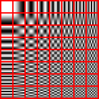
The values closer to the upper-left corner of the matrix are more significant, and values approach 0 further to the bottom-right.
This is due to the nature of the DCT, preserving coarser information in the upper left and removing fine information not perceivable by humans. Here is the DCT below:

Image taken from Wiki
Entropy Coding
This step is used to convert our matrix into a sequence of integers, by passing over the array across its diagonals from top left to bottom right (in a “zig-zag” pattern).
This is because, we are more likely to see integers at the top-left, and therefore when we compact this data, the RLE will be more optimised.
Run Length Encoding (RLE)
Essentially, we take our 1D array of data, and instead of writing values like 0, 0, 0, we write them like 0[x3] to save space. This has a significant part in the result and is often used on all sorts of data. In fact, I will be learning about RLE in my EPQ project to come. (It is related to Cellular Automata and is a file format used to store patterns. Learn more here)
Huffman Encoding
This is a separate encoding algorithm which assigns shorter bit codes to the more frequent values in our data, and longer codes to the less frequent. This results in an even higher degree of compression. (This is quite a complex topic, and if you want to learn more about this and other algorithms, you can do so with this book by Thomas H. et al. (pg. 431))
Decoding Our JPEG
In order to decode our JPEG, we can simply follow all of these steps in reverse. We start by decoding our image, through a Huffman decoder, and our Run Length Decoder. Once we’ve done this, we can convert our 1D array of values into a 2D image by “unravelling” the zig-zag pattern. We know the dimensions of the image because this is stored in the metadata of the image (As well as other important information such as which quality/quantisation table was used).
Our matrix is then multiplied with the quantisation table using a Hadamard product (element-wise) denoted as:
$$\text{Image} \odot Q$$
Which is as close to the reverse of the above step:
np.round(np.divide(dct, Q))
Which performs Hadamard division with rounding.
$$\text{Quantised result} = \text{round(}dct\oslash Q)$$
Once we have done this, all we need to do is convert our image back into the RGB colour space, with a simple Y'CbCr to RGB conversion. This can be done using OpenCV and the cv2.COLOR_YCrCb2RGB Function:
rgb = cv2.cvtColor(dct, cv2.COLOR_YCrCb2RGB)
And we should have our image.
Optimisations
There are plenty of ways to optimise this, one of the more notable optimisations was performed by the developers at libjpeg-turbo, who have accelerated the encoding and decoding of JPEGs using Single Instruction, Multiple Data (SIMD) Instructions, as well as optimised Huffman coding routines.
With this, It can perform 2-6x as fast as libjpeg. You can find the GitHub repository here
That’s All
Thank you very much for reading.
I recommend taking a look at all the above links, as well as this PDF with an explanation of all the technical terms.
Expect to see Blog posts quarterly with more exciting topics on the way. As 2023 goes on, I may expand these articles, so do check back if you’re interested.
I’m open to any feedback you may have. Please do not hesitate to get in contact via email if you have any queries.
Subscribe to my newsletter
Read articles from Olivier Hinds directly inside your inbox. Subscribe to the newsletter, and don't miss out.
Written by

Olivier Hinds
Olivier Hinds
I'm a passionate Software Developer with a keen interest in becoming a Mechanical Engineer. My journey in software development has been a crucial stepping stone towards this goal, enhancing my skills and preparing me for the exciting challenges that lie ahead.