Getting Started with Machine Learning in Python - Part 1 of 2.

Machine learning is a computer science field where computer systems give sense to data in a similar way to human beings. It is an artificial intelligence type that extracts patterns from raw data through algorithms. Machine learning enables computer systems to gain experience without human intervention or programming.

In the tutorial, we are going to learn the various methods of machine learning, how to load data, understanding data and data preparation.

Machine Learning methods

They include:

Supervised Learning

Supervised learning algorithms takes the training data and the related output during the process of training. For instance, when we have x input variables and y output variables, we apply the algorithm as follows

y = f(x)

Unsupervised Learning

Unsupervised learning is the opposite of supervised learning. It means the machine learning algorithms lack supervisors to give guidance.

Reinforcement Learning

In reinforcement learning, an agent receives training over a particular time period for it to interact with caertain environment. After observing the environment, the agent then takes action concerning the present state of the environment.

Loading Data

The Python script for loading CSV data file using Pandas on Pima Indians Diabetes dataset is given below

from pandas import read_csv
from matplotlib import pyplot
import numpy as np
import pandas as pd
path = r"C:\Users\User\Documents\DATA ANALYST\Datasets\pima-indians-diabetes.csv"
data = read_csv(path)
print(data[:3])

Understanding data with statistics

Data dimensions

It is important to know data in terms of columns and rows. Much data takes much time to run algorithms and train the model. On the other hand, less data does not provide enough information to train the model.

print(data.shape)

We can then proceed to look at the data summary.

print(data.describe)

Understanding data with visualization

Data visualization can assist us in knowing what data looks like and the type of correlation between data attributes. It is the quickest way of seeing whether the characteristics relate to the output.

Data visualization techniques include univariate plots and multivariate plots

Univariate Plots

Examples of univariate plots are histograms, density plots, and box plots

Histogram

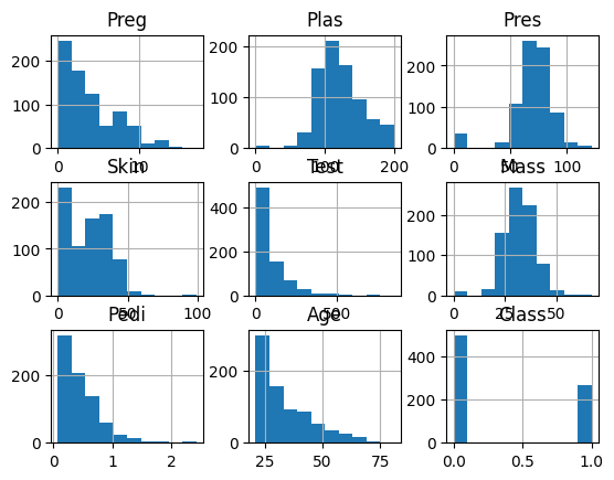
Python script to create Pima Indian Diabetes dataset attributes histogram using hist() function on Pandas DataFrame to generate histograms and matplotlib for plotting them.

data.hist()
pyplot.show()

Density Plot

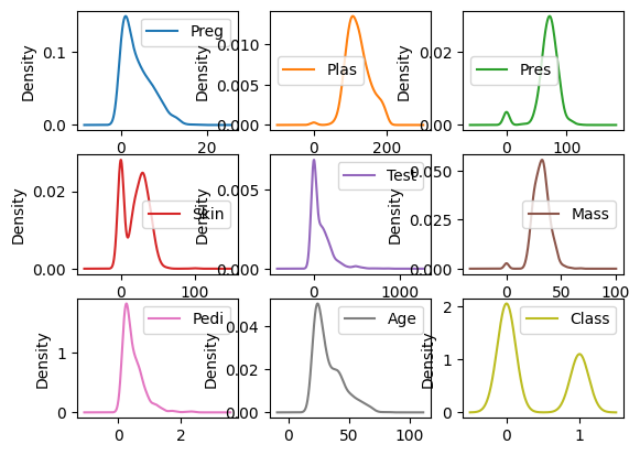
Density plots are easy and quick techniques for getting each distribution attributes with a smooth curve through the top of every bin. Python script will generate Density Plots for the distribution of attributes of the Pima Indian Diabetes dataset

data.plot(kind='density', subplots=True, layout=(3,3), sharex=False)
pyplot.show()

Box Plot

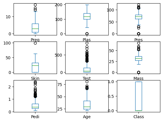
Python script to generate box plots for the distribution of attributes of Pima Indian Diabetes dataset.

data.plot(kind='box', subplots=True, layout=(3,3), sharex=False,sharey=False)
pyplot.show()

Multivariate Plots

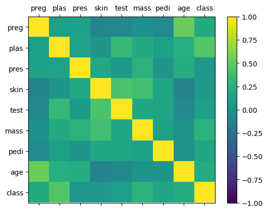
Multivariate plots are correlation matrix plots.

Python script to generate and plot correlation matrix for the Pima Indian Diabetes dataset uses corr() function on Pandas DataFrame and plotted with the help of pyplot

names = ['preg', 'plas', 'pres', 'skin', 'test', 'mass', 'pedi', 'age', 'class']
data = read_csv(path)
correlations = data.corr()
fig = pyplot.figure()
ax = fig.add_subplot(111)
cax = ax.matshow(correlations, vmin=-1, vmax=1)
fig.colorbar(cax)
ticks = np.arange(0,9,1)
ax.set_xticks(ticks)
ax.set_yticks(ticks)
ax.set_xticklabels(names)
ax.set_yticklabels(names)
pyplot.show()

Data Preparation

Data preprocessing converts data to a form we can work with or can feed to ML algorithms. The data preprocessing techniques include standardization, scaling, normalization, and binarization.

Scaling

Data rescaling ensures data is on the same scale since dataset attributes have varying scales. Attributes are generally rescaled to 0-1 range. We will rescale the data of Pima Indians Diabetes dataset.

from pandas import read_csv
from numpy import set_printoptions
from sklearn import preprocessing
array = data.values

We can rescale data using MinMaxScaler

data_scaler = preprocessing.MinMaxScaler(feature_range=(0,1))
data_rescaled = data_scaler.fit_transform(array)

We can also summarize data output according to our choice. We will set the precision to 1 and show the first 10 rows in the output.

set_printoptions(precision=1)
print ("\nScaled data:\n", data_rescaled[0:10])

Normalization

The data preprocessing technique is used to rescale each row of data to have a length of 1

L1 Normalization

The normalization technique modifies dataset values in a way that the total absolute values in every row are 1. It is known as the Least Absolute Deviations.

from sklearn.preprocessing import Normalizer
Data_normalizer = Normalizer(norm='l1').fit(array)
Data_normalized = Data_normalizer.transform(array)
set_printoptions(precision=2)
print ("\nNormalized data:\n"), Data_normalized [0:3]

L2 Normalization

L2 normalization technique modifies dataset values in a way that the sum of squares in each row the sum of the squares will always be up to 1. It is also called least squares.

from sklearn.preprocessing import Normalizer
Data_normalizer = Normalizer(norm='l2').fit(array)
Data_normalized = Data_normalizer.transform(array)
set_printoptions(precision=2)
print ("\nNormalized data:\n", Data_normalized [0:3])

Binarization

The binary threshold is used for making data binary whereby the values above the threshold are converted to 1 while values below the threshold are converted to 0. The technique is mostly used when there are probabilities in the dataset that require conversion to crisp Values.

from sklearn.preprocessing import Binarizer
binarizer = Binarizer(threshold=0.5).fit(array)
Data_binarized = binarizer.transform(array)
print ("\nBinary data:\n", Data_binarized [0:5])

Standardization

The technique is used in transforming the data attributes with a Gaussian distribution. It differs the mean and Standard Deviation (SD) to a standard Gaussian distribution with a mean of 0 and a SD of 1. This technique is useful in ML algorithms like linear regression, logistic regression that assumes a Gaussian distribution in input dataset and produce better results with rescaled data.

from sklearn.preprocessing import StandardScaler
data_scaler = StandardScaler().fit(array)
data_rescaled = data_scaler.transform(array)
set_printoptions(precision=2)
print ("\nRescaled data:\n", data_rescaled [0:5])

Data Labelling

Most of the sklearn functions expect data with number labels rather than word labels. Therefore, there is a need to convert such labels into number labels. We can perform label encoding of data with the help of LabelEncoder() function.

For example, input values can be:

input_labels = ['red','black','red','green','black','yellow','white']

The next line of code will create the label encoder and train it

encoder = preprocessing.LabelEncoder()
encoder.fit(input_labels)

We can check performance by encoding a random ordered list

test_labels = ['green','red','black']
encoded_values = encoder.transform(test_labels)
print("\nLabels =", test_labels)
print("Encoded values =", list(encoded_values))
encoded_values = [3,0,4,1]
decoded_list = encoder.inverse_transform(encoded_values)

We can get the list of encoded values using the following Python script

print("\nEncoded values =", encoded_values)
print("\nDecoded labels =", list(decoded_list))

Feature Selection Techniques

Machine learning functionality has direct proportionality to features of training data. Automatic feature selection is the process of selecting the most relevant data features to output variable. The importance of conducting automatic feature selection before modeling data includes reducing overfitting, increasing the ML model's accuracy, and decreasing training time.

The automatic feature techniques that can be used in modeling machine learning data in Python include univariate selection and recursive feature elimination.

Univariate Selection

The technique is used in choosing features with the assistance of statistical testing and SelectKBest0class of the scikit-learn Python library.

For instance, we utilize Pima Indians Diabetes dataset to choose 4 attributes with the best features using a chi-square statistical test.

from pandas import read_csv
from numpy import set_printoptions
from sklearn.feature_selection import SelectKBest
from sklearn.feature_selection import chi2
dataframe = read_csv(path)
array = dataframe.values

We will then separate the array into input and output components

X = array[:,0:8]
Y = array[:,8]

The Python script below selects the best features from the dataset

test = SelectKBest(score_func=chi2, k=4)
fit = test.fit(X,Y)

We can also summarize the data for output as per our choice. Here, we are setting the precision to 2 and showing the 4 data attributes with best features along with best score of each attribute −

set_printoptions(precision=2)
print(fit.scores_)
featured_data = fit.transform(X)
print ("\nFeatured data:\n", featured_data[0:4])

[ 111.52 1411.89 17.61 53.11 2175.57 127.67 5.39 181.3 ]
Featured data:
[
   [148. 0.  33.6 50. ]
   [ 85. 0.  26.6 31. ]
   [183. 0.  23.3 32. ]
   [ 89. 94. 28.1 21. ]
]

Recursive Feature Elimination

The technique recursively removes attributes and creates a model with the attributes that remain. We can implement RFE feature selection technique using RFE class of scikit-learn Python library.

We can use RFE with a logistic regression algorithm in selecting the best 3 attributes with the best features from Pima Indians Diabetes dataset.

from sklearn.feature_selection import RFE
from sklearn.linear_model import LogisticRegression
dataframe = read_csv(path)
array = dataframe.values

We will then separate the array into input and output components

X = array[:,0:8]
Y = array[:,8]

The code below selects the best features from a dataset

model = LogisticRegression()
rfe = RFE(model, 3)
fit = rfe.fit(X, Y)
print("Number of Features: %d")
print("Selected Features: %s")
print("Feature Ranking: %s")

Number of Features: 3
Selected Features: [ True False False False False True True False]
Feature Ranking: [1 2 3 5 6 1 1 4]

From the output, the selected best features are preg, mass, and pedi. They are marked as 1 in the output.

Principal Component Analysis (PCA)

The data reduction technique is a beneficial feature selection technique that utilizes linear algebra in compressing datasets. We can implement the technique using PCA class of scikit-learn Python library.

from sklearn.decomposition import PCA

We will then separate array into input and output components

X = array[:,0:8]
Y = array[:,8]

The Python script that extracts features from dataset is given below

pca = PCA(n_components=3)
fit = pca.fit(X)
print("Explained Variance: %s") % fit.explained_variance_ratio_
print(fit.components_)

Explained Variance: [ 0.88854663 0.06159078 0.02579012]
[
   [ 
      -2.02176587e-03 9.78115765e-02 1.60930503e-02 6.07566861e-02 
      9.93110844e-01 1.40108085e-02 5.37167919e-04 -3.56474430e-03
   ]
   [ 
      2.26488861e-02 9.72210040e-01 1.41909330e-01 -5.78614699e-02 
      -9.46266913e-02 4.69729766e-02 8.16804621e-04 1.40168181e-01
   ]
   [ 
      -2.24649003e-02 1.43428710e-01 -9.22467192e-01 -3.07013055e-01 
      2.09773019e-02 -1.32444542e-01 -6.39983017e-04 -1.25454310e-01
   ]
]

We can observe from the above output that 3 Principal Components bear little resemblance to the source data.

Feature Importance

The technique is used in selecting important features and uses trained supervised classifier in selecting features.

The technique can be implemented using ExtraTreeClassifier class of scikit-learn Python library.

For instance, we will use ExtraTreeClassifier to select features from Pima Indians Diabetes dataset.

from sklearn.ensemble import ExtraTreesClassifier

Next, we will separate the array into input and output components

X = array[:,0:8]
Y = array[:,8]

The following lines of code will extract features from dataset

model = ExtraTreesClassifier()
model.fit(X, Y)
print(model.feature_importances_)

[ 0.11070069 0.2213717 0.08824115 0.08068703 0.07281761 0.14548537 0.12654214 0.15415431]

From the output, we can observe that there are scores for each attribute. The higher the score, the higher the importance of that attribute.

Conclusion

We have learned how to get started with machine learning in Python where we have covered the necessary Python libraries we need to install, how to load data, various machine learning methods, understanding data with statistics, and understanding data with visualization. Also, we have learned how to prepare machine learning data with data preprocessing techniques such as standardization, scaling, normalization, and binarization. Lastly, we have covered feature selection techniques including univariate selection, recursive feature elimination, principal component analysis and feature importance. In the next article, we will cover machine learning algorithms such as classification, regression, clustering, and KNN algorithm.

Thany you for reading the article. I hope it has been beneficial to you as you begin machine learning journery.