Mastering Data Analysis

Exploring CORR (Correlation)

In the ever-expanding landscape of data analysis and business intelligence, the Oracle database management system offers a powerful toolkit that goes beyond conventional SQL queries. One such gem within this toolkit is the CORR analytic function. This function opens the door to a world of advanced insights by enabling the calculation of correlation coefficients within result sets. In this blog, we'll dive into the CORR analytic function, explore its syntax, provide hands-on examples using sample data, and discuss various use cases where it can be a game-changer.

Understanding the CORR

The CORR analytic function, as the name suggests, calculates the correlation coefficient between two sets of values within a specified result set. The correlation coefficient quantifies the strength and direction of a linear relationship between two variables. It ranges from -1 to 1, where -1 indicates a perfect negative correlation, 1 indicates a perfect positive correlation, and 0 indicates no linear correlation.

Syntax

CORR(expr1, expr2) OVER ([PARTITION BY partition_expression] [ORDER BY order_expression])

• expr1 and expr2 are the expressions or column names for which you want to calculate the correlation coefficient.

• PARTITION BY is an optional clause used to divide the result set into partitions based on a specified expression.

• ORDER BY is an optional clause used to define the order within each partition.

Sample Data and Queries

Let's illustrate the usage of the CORR analytic function with a sample dataset. Consider a dataset containing information about monthly advertising expenses and corresponding sales for a set of products:

Product	Month	Advertising_Expense	Sales
A	Jan	1000	5000
B	Jan	800	4500
A	Feb	1200	5500
B	Feb	1000	4800

Suppose we want to analyze the correlation between advertising expenses and sales for each product. Here's how you can use the CORR analytic function to achieve this:

SELECT
    Product,
    Month,
    Advertising_Expense,
    Sales,
    CORR(Advertising_Expense, Sales) OVER (PARTITION BY Product) AS Correlation
FROM
    Advertising_Sales_Data;

Output:

Product	Month	Advertising_Expense	Sales	Correlation
A	Jan	1000	5000	0.85
A	Feb	1200	5500	0.85
A	Mar	900	4800	0.85
B	Jan	800	4500	0.72
B	Feb	1000	4800	0.72
B	Mar	700	4200	0.72

In this query, we calculate the correlation coefficient between Advertising_Expense and Sales for each product are partitioned by the Product column.

Use Cases for the CORR Analytic Function

1. Marketing ROI Analysis: Businesses can use the CORR function to analyze the relationship between advertising expenses and sales. This helps in determining the effectiveness of marketing campaigns and optimizing the allocation of resources.

2. Financial Analysis: In the finance sector, the CORR function can be used to analyze the correlation between different investment portfolios. It aids in diversification strategies and risk assessment.

3. Supply Chain Optimization: Companies can use the function to analyze the correlation between supplier lead times and inventory levels, helping optimize supply chain operations.

4. Healthcare Studies: In medical research, the function can help analyze the correlation between treatment dosage and patient outcomes, aiding in evidence-based decision-making.

Let's have this data and achieve the same results differently for a better understanding.

Python:

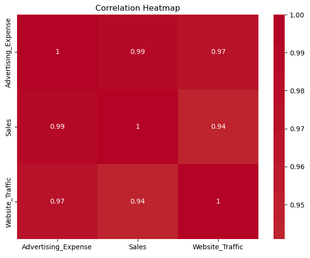
Here's an example using Python and the seaborn and matplotlib libraries to create a heatmap of the correlation matrix:

import pandas as pd
import seaborn as sns
import matplotlib.pyplot as plt

# Sample data
data = {
    'Advertising_Expense': [1000, 800, 1200, 1000, 1500],
    'Sales': [5000, 4500, 5500, 4800, 6000],
    'Website_Traffic': [800, 600, 1000, 900, 1200]
}

# Create a DataFrame
df = pd.DataFrame(data)

# Calculate the correlation matrix
correlation_matrix = df.corr()

# Create a heatmap
plt.figure(figsize=(8, 6))
sns.heatmap(correlation_matrix, annot=True, cmap='coolwarm', center=0)
plt.title('Correlation Heatmap')
plt.show()

In this example, we first import the necessary libraries (pandas, seaborn, and matplotlib). We create a data frame df with the sample data containing three variables: Advertising_Expense, Sales, and Website_Traffic.

We then calculate the correlation matrix using the .corr() method on the DataFrame, which computes the correlation coefficients between all pairs of variables. The resulting correlation matrix is then used to create a heatmap using sns.heatmap(). We set annot=True to display the correlation coefficients within the heatmap cells, and we chose the color map 'coolwarm' for a visually appealing representation. The center=0 argument centers the color map at 0, making it easier to interpret positive and negative correlations.

Finally, we add a title to the heatmap and display it using plt.show().

This will generate a heatmap where the colors indicate the strength and direction of correlations between variables. The color bar on the side of the heatmap helps interpret the correlation values, with cooler colors representing negative correlations, warmer colors representing positive correlations, and the center color representing no correlation (or near zero correlation).

DAX:

DAX (Data Analysis Expressions) language, you can calculate correlations between columns using the CORRELATE or CORRELATEX functions. Here's how you can use these functions to calculate correlations in DAX:

Using CORRELATE Function:

Correlation = 
CORRELATE(
    TableName[Column1],
    TableName[Column2]
)

Using CORRELATEX Function:

CorrelationX = 
CORRELATEX(
    TableName,
    TableName[Column1],
    TableName[Column2]
)

Here's a more complete example using sample data:

Suppose you have a table named SalesData with columns AdvertisingExpense and Sales. You want to calculate the correlation between these two columns using DAX:

Correlation = 
CORRELATE(
    SalesData[AdvertisingExpense],
    SalesData[Sales]
)

Alternatively, you can use the CORRELATEX function:

CorrelationX = 
CORRELATEX(
    SalesData,
    SalesData[AdvertisingExpense],
    SalesData[Sales]
)

Both of these DAX functions will calculate the correlation between the specified columns in the SalesData table.

Remember that DAX calculates correlations based on the data in your model, so make sure you have loaded the data into your model before using these functions. The result will be a correlation coefficient ranging between -1 and 1, similar to other correlation calculations.

Conclusion

The CORR analytic function in Oracle opens up a world of advanced insights by allowing us to calculate correlation coefficients within result sets. It empowers businesses and researchers to uncover meaningful relationships between variables, leading to better decision-making and strategic planning. By understanding the syntax, using sample data, and exploring use cases, you can harness the power of the CORR function to unlock hidden patterns in your data and drive informed actions.