Greedy Algorithms and Optimization Problems
 Akash Dev
Hey, dear readers! 👋 Welcome to the third article in my blog series. If you haven't read my previous articles, I recommend checking those out first. However, you can also start right here, as I'll be explaining everything from scratch.
Introduction
In the world of algorithms and problem-solving, we often turn to greedy algorithms when faced with optimization challenges. These are situations where we aim to minimize or maximize some value—whether it's cost, profit, weight, count, or something else entirely.
Note: It's important to remember that while greedy algorithms are powerful, they don't always guarantee an optimal solution. In cases where optimality is critical, we turn to dynamic programming. But don't worry, my next article will delve into the world of dynamic programming, so stay tuned for that!
Problems Based on Greedy Algorithms
Now, let's explore some fascinating problems that can be tackled using greedy algorithms:
Coin Exchange Problem
Imagine you need to make a certain amount of money N using the least number of coins from a given set of denominations D = {d1, …, dn}. Let's take the Indian coin system as an example: {5, 10, 20, 25, 50, 100}.
Suppose we want to give change for 40 paisa. We can solve this problem by repeatedly choosing a coin that's less than or equal to the current amount, resulting in a new amount. In the greedy algorithm, we always select the largest possible coin value without exceeding the total amount. For instance, for 40 paise, the greedy algorithm gives us coins {25, 10, and 5}, but the optimal solution is {20, 20}.
Here's a Python function to implement this:
def make_change(N):
    C = [5, 20, 25, 50, 100]  # Constant denominations
    S = []  # Set that will hold the solution set
    Value = N

    while Value != 0:
        x = max(item for item in C if item < Value)
        if x is None:
            return "No Solution"
        S.append(x)
        Value -= x

    return S
Minimum Spanning Tree
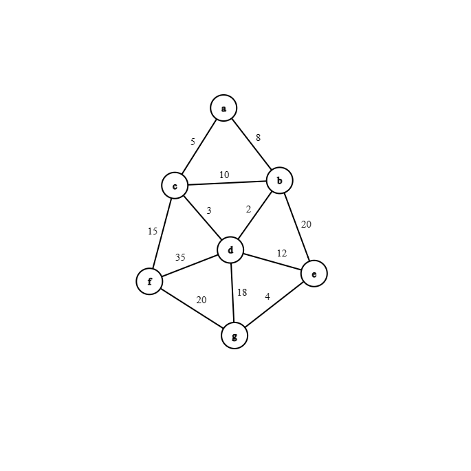
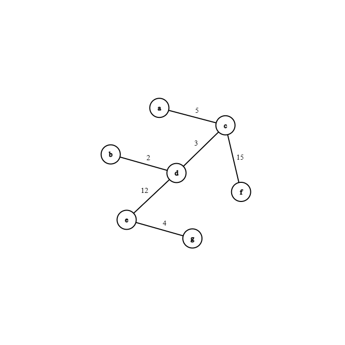
A spanning tree of a connected graph is a tree that includes all the vertices. A minimum spanning tree (MST) of a weighted graph is a spanning tree with the smallest possible sum of edge weights.

Graph

Minimum spanning tree
Prim's Algorithm
Prim's algorithm constructs a single tree T one edge at a time, gradually forming a spanning tree. We start with T having zero edges and a set U containing a single node. At each step, Prim’s algorithm adds the smallest weighted edge with one endpoint in U and the other not in U. After n-1 additions, U contains all the vertices of the spanning tree, and T becomes an MST.
Here's a Python function to implement Prim's Algorithm:
def prim(graph):
    T = {}
    r = any_vertex_in_graph(graph)
    U = {r}

    for i in range(1, len(graph.vertices)):
        e = minimum_weight_edge(graph, U)
        U.add(e.v)
        T.add(e)

    return T
Prim’s Algorithm uses a priority queue (min-heap) to get the closest fringe vertex, and it has a time complexity of O(m log n), where n is the number of vertices and m is the number of edges in the MST.
Kruskal's Algorithm
Kruskal’s Algorithm is another method to create a minimum spanning tree. It constructs the MST by choosing the smallest weighted edge that doesn't form a cycle and repeats this process until all the edges from the original set are exhausted.
Here's a Python function to implement Kruskal's Algorithm:
def kruskal(graph):
    sort_edges(graph.edges)  # Sort the edges by weight
    T = set()

    while len(T) + 1 < len(graph.vertices):
        e = next_edge(graph.edges)
        if not creates_cycle(T, e):
            T.add(e)

    return T
Kruskal’s Algorithm has a time complexity of O(E log V) using efficient cycle detection.
Dijkstra’s Algorithm
Dijkstra’s algorithm is used for the single-source shortest path problem with weighted edges having no negative weights. It determines the length of the shortest path from a source vertex to all other nodes in the graph.
Here's a Python function to implement Dijkstra's Algorithm:
import heapq

def dijkstra(graph, source):
    D = {}
    P = {}
    PQ = []

    for v in graph.vertices:
        D[v] = float('inf')  # Unknown distance
        P[v] = None  # Unknown previous node
        heapq.heappush(PQ, (D[v], v))

    D[source] = 0  # Distance from source to source

    while PQ:
        _, u = heapq.heappop(PQ)

        for v in graph.adjacent_vertices(u):
            alt = D[u] + graph.edge_length(u, v)
            if alt < D[v]:
                D[v] = alt
                P[v] = u

    return D, P
Dijkstra’s Algorithm has a time complexity of O(|E| log |V|).
Huffman Trees for Optimal Encoding
Encoding assigns bit strings to alphabet characters. Two types of encoding are fixed-length encoding (e.g., ASCII) and variable-length encoding (e.g., Huffman code). Huffman codes are the best prefix-free codes. No code word is a prefix of another code word, making them optimal for compression.
Huffman’s algorithm constructs a binary tree whose leaf values are assigned optimal codes for text compression. The most frequent words get smaller Huffman codes.
Here's a Python function to implement Huffman's Algorithm:
import heapq

def huffman(C, W):
    PQ = []

    for i in range(len(C)):
        T = TreeNode()
        T.char = C[i]
        T.weight = W[i]
        heapq.heappush(PQ, (W[i], T))

    for i in range(len(C) - 1):
        L = heapq.heappop(PQ)
        R = heapq.heappop(PQ)
        T = TreeNode()
        T.add_children(L, R)
        T.weight = L.weight + R.weight
        heapq.heappush(PQ, (T.weight, T))

    return PQ[0][1]
Huffman’s Algorithm has a time complexity of O(n log n).
Activity Selection Problem
Introduction: The activity selection problem involves selecting a non-overlapping set of activities from a given set of activities, each with defined start and finish times. The goal is to maximize the number of activities scheduled.
Problem Statement: Given a set of activities S = {a1, a2, ..., an}, each activity ai needs a resource during the time period [si, fi), where si is the start time
and fi is the finish time. Activities are sorted in increasing order of finish times, i.e., f1 ≤ f2 ≤ ... ≤ fn-1 ≤ fn.
Example: Consider these activities:
| Activity | 1 | 2 | 3 | 4 | 5 | 6 | 7 | 8 | 9 | 10 | 11 |
| Start | 1 | 3 | 0 | 5 | 3 | 5 | 6 | 8 | 8 | 2 | 11 |
| Finish | 4 | 5 | 6 | 7 | 8 | 9 | 10 | 11 | 12 | 13 | 14 |
We want to find the maximum number of non-overlapping activities. An optimal solution is {a1, a3, a6, a8}, maximizing the number of activities scheduled.
Algorithm:
def ActivitySelection(S, F, N):
    # Sort activities by finish time
    Sort(S, F)
    A = [a1]
    K = 1
    for m in range(2, N + 1):
        if S[m] >= F[K]:
            A.append(am)
            K = m
    return A
Knapsack Problem
Fractional Knapsack Problem
Introduction: Imagine a thief trying to maximize profit by stealing items from a store. Each item has a cost and a weight, and the thief's knapsack has a maximum weight capacity. In this scenario, the thief can take fractions of items.
Algorithm:
def FractionalKnapsack(W, C, Wk):
    for i in range(1, n + 1):
        X[i] = 0
    Weight = 0
    # Use Max heap
    H = BuildMaxHeap(C/W)
    while Weight < Wk:
        i = H.GetMax()
        if Weight + W[i] <= Wk:
            X[i] = 1
            Weight = Weight + W[i]
        else:
            X[i] = (Wk - Weight) / W[i]
            Weight = Wk
    return X
0/1 Knapsack Problem
Introduction: In the 0/1 Knapsack Problem, the thief can either take an entire item or leave it. Fractional strategies like the ones above won't work, and a greedy approach could lead to suboptimal solutions.
Algorithm: This problem is typically solved using dynamic programming, which will be covered in a future article.
In this article, I've talked about the world of greedy algorithms, and their power to solve optimization problems. If you found this article helpful don't forget to hit that like button and if you were unable to understand anything just tell me in the comments below.
Don't miss out on more algorithmic insights! Catch up on our previous articles and stay updated by subscribing to our newsletter. 🚀💡
Happy coding!
Subscribe to my newsletter
Read articles from Akash Dev directly inside your inbox. Subscribe to the newsletter, and don't miss out.
Written by

Akash Dev
Akash Dev
Hello! My name is Akash Dev and I am a computer science student with a passion for technology. I started this blog as a way to document my learning journey and share my knowledge and insights with others who are also interested in the field of computer science. I cover a wide range of topics including programming languages, software development, and emerging technologies. I hope my blog will be a valuable resource for anyone looking to learn more about computer science and technology. Join me as I explore the fascinating world of computer science and discover new things together.