In the previous part, we delved into various fundamental statistical concepts such as mean, mode, median, skewness, variance, and more. Today, we're going to continue our exploration of statistical knowledge by delving into several other crucial topics in the field of statistics like Sampling Distribution, Central Limit Theorem(CLT), and up to Estimators.

Inferential Statistic👇

Inferential statistics refers to a method that relies on probability and distribution in particles to predict population values based on sample data.

Distribution👇

A distribution is a function that shows the possible values for a variable and how often they occur.

If all outcomes have an equal chance of occurring that’s called Discrete uniform distribution.

Each probability distribution has a visual representation, It is a graph describing the likelihood of occurrence of every event.

A distribution is defined by the underlying probabilities and not the graph. The graph is just a visual representation.

The Normal DIstribution👇

Experienced statisticians can immediately distinguish a binomial from a Poisson distribution as well as a uniform exponential distribution in a quick glimpse at a plot.

Why Normal or Student-T distribution?👇

1. They approximate a wide variety of random variables

2. Distributions of sample mean with large enough sample sizes could be approximated to normal.

3. All computable statistics are elegant.

4. Decisions based on normal distribution insights have a good track record.

Graph of Normal Distribution👇

The Normal distribution is the most common.

The statistical term of Normal distribution graphs is Gaussian Distribution bell-shaped.

It is symmetrical and the normal distribution is the most commonly used. mean, median and mode are equal.

Normal Distribution is defined by -

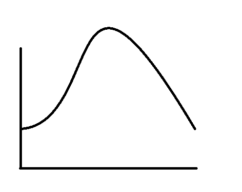
The highest point of the graph is located at the mean because it coincides with the mode.

The spread of the graph is determined by the standard deviation.

A lower mean would result in the same shape of the distribution, but on the left side of the plane, like -

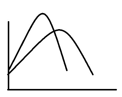
The bigger man would move the graph to the right.

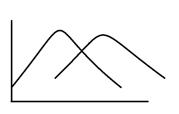
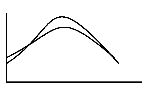
A lower standard deviation results in a lower dispersion. So more data in the middle and thinner tails.

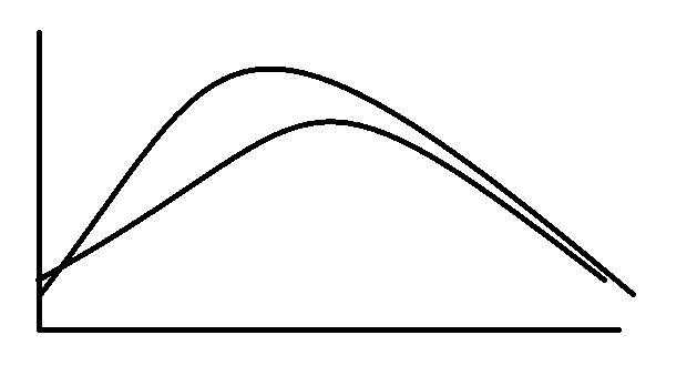
A higher standard deviation will cause the graph to flatter out with fewer points in the middle and more to the end, or fatter tails in statistics jargon.

The Standard Normal Distribution👇

Every distribution can be standardized.

Standardization transforms this variable into one with a mean of 0 and a standard deviation of 1.

Logically, a normal distribution can also be standardized, the result is called a standard normal distribution.

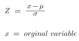
If we shift the mean by mu and the standard deviation by sigma for any normal distribution, we will arrive at the standard normal distribution.

We use the letter ‘Z’ to denote the standard normal distribution, so -

The standardized variable is called the z-score.

Sampling Distribution Or Central Limit Theorem(CLT)👇

If we want to predict the same can prices. In this case, population parameters that may be of interest are mean car price. The standard deviation of prices, covariance, and so on.

Normally in statistics, we would not have data on the whole population, but rather just a sample.

On sample data, the sample mean depends on the incumbents of the sample itself.

Taking a single value as we did in descriptive statistics is defining suboptimal.

Examples-

2154.49	2623.52	2786.31
2551.55	2661.13	2804.30
2568.22	2687.14	2844.82
2594.64	2711.35	3030.01
25617.23	2744.97	3201.34
2620.85	2748.44	3248.88

These values are distinct in some way so we have a distribution

When we are referring to a distribution form by samples, we use the term sampling distribution.

In our case, we can be even more precise, we are dealing with a sampling distribution of the mean.

Distribution of car prices-

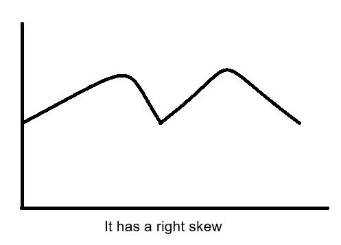
If we visualize the distribution of the sampling mean, we get something else, something familiar, something useful, a normal distribution, and that is what the central limit theorem states, No matter whether the distribution of the population is binomial, uniform, exponential, or another one.

The sampling distribution of the mean will approximate a normal distribution.

Its mean is the same as the population means and variance depends on the size of the sample we draw but it’s quite elegant.

it‘s the population variance divided by the sample size(n).

Usually, for CLT(Central Limit Theorem) to apply, we need a sample size of at least 30 observations (n>30)

Why CLT?👇

Because CLT allows us to perform tests, solve problems, and make inferences using the normal distribution, even when the population is not normally distributed.

Standard Error👇

What is Standard error?👇

The standard error is the standard deviation of the distribution formed by the sample means. In other words, the standard deviation of the sampling distribution.

The standard deviation of the sampling distribution is -

Like a standard deviation, the standard error shows variability. In this case, it is the variability of the means of the different samples we extracted.

What is it important?👇

Because it’s used for almost all statistical tests because it shows how well you approximated the true mean.

Note: It decreases as the sample size increases.

Estimator And Estimates👇

What is Estimator?👇

The estimator of a population parameter is an approximation depending solely on sample information, A specific value is called an estimate.

There are two types of estimates

1. Point estimate

2. Confidence interval estimate

What is a Point Estimate?👇

A point estimate is a single number while a confidence interval is an interval two are closely related. The point estimates are located exactly in the middle of the confidence interval.

Confidence intervals provide much more information and are preferred for making inferences

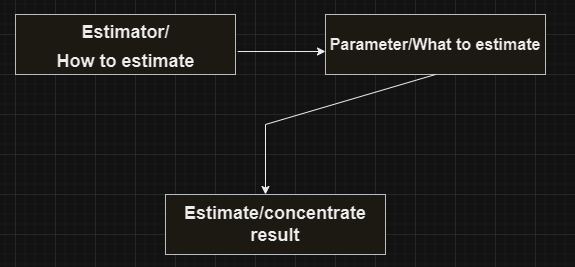
There may be many estimators for the same variable.

They all have two properties -

1. Bias

2. Efficiency

Estimators are like judges. 

We are always looking for the most efficient unbiased estimators.

An unbiased estimator has an expected value equal to the population parameter

If someone says you will find the average height of Americans by taking a sample, finding its mean, and then adding 1 foot to that result the formula is -

Bias:

Efficiency:

The most efficient estimators are the ones with the least variability of outcomes.

The most efficient estimator is the unbiased estimator with the smallest variance.

What is the difference between estimators and statistics?👇

• The word statistic is the broader term

• A point estimate is a type of statistic

Before we end…

Thank you for taking the time to read my posts and share your thoughts. If you like my blog please give a like, comment, and share it with your circle and follow for more I look forward to continuing this journey with you.

Let’s connect and grow together. I look forward to getting to know you better😉.

Here are my social links below-

Linkedin: https://www.linkedin.com/in/ai-naymul/

Twitter: https://twitter.com/ai_naymul

Github: https://github.com/ai-naymul