Understanding Overfitting, Underfitting, Bias, and Variance

Machine learning models are powerful tools that can uncover patterns and insights from data. Creating a model that accurately predicts outcomes is the ultimate goal. However, finding the right balance between a model that is too simple and one that is too complex can be challenging. Overfitting and underfitting are common challenges encountered in the process of model training, while bias and variance are key concepts that help us understand the performance of our models.

Overfitting:

Overfitting occurs when a model learns the training data too well, capturing noise or random fluctuations that are not representative of the true underlying patterns. This can lead to poor generalization performance on new, unseen data.

Underfitting:

Conversely, underfitting occurs when a model is too simplistic and fails to capture the underlying patterns in the data. An underfit model performs poorly both on the training and new data.

Bias:

Bias is an error introduced by approximating a real-world problem too simplistically. High bias can lead to underfitting.

Variance:

Variance is the amount by which the model's predictions would change if it were trained on a different dataset. High variance can lead to overfitting.

In practice, finding the right balance between overfitting and underfitting involves techniques like cross-validation, regularization, and using appropriate model complexity.

Let's consider a polynomial regression problem. Suppose you have a dataset that follows a quadratic trend, but you fit a linear regression model to it.

import numpy as np
import matplotlib.pyplot as plt
from sklearn.model_selection import train_test_split
from sklearn.linear_model import LinearRegression
from sklearn.preprocessing import PolynomialFeatures
from sklearn.metrics import mean_squared_error

# Generate synthetic data
np.random.seed(42)
X = np.sort(5 * np.random.rand(80, 1), axis=0)
y = 3 * X.squeeze()**2 + np.random.randn(80) * 1.5

# Split the data
X_train, X_test, y_train, y_test = train_test_split(X, y, test_size=0.2, random_state=42)

# Fit a linear regression model
model_linear = LinearRegression()
model_linear.fit(X_train, y_train)

# Fit a quadratic (degree=2) regression model
poly_features = PolynomialFeatures(degree=2, include_bias=False)
X_train_poly = poly_features.fit_transform(X_train)
model_quadratic = LinearRegression()
model_quadratic.fit(X_train_poly, y_train)

# Visualize the results
X_range = np.arange(0, 5, 0.01)[:, np.newaxis]
y_pred_linear = model_linear.predict(X_range)
y_pred_quadratic = model_quadratic.predict(poly_features.transform(X_range))

plt.scatter(X, y, color='blue', label='Data points')
plt.plot(X_range, y_pred_linear, color='red', label='Linear Regression')
plt.plot(X_range, y_pred_quadratic, color='green', label='Quadratic Regression')
plt.title('Linear vs. Quadratic Regression')
plt.legend()
plt.show()

Output

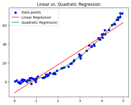
In the above example, fitting a linear model (in red) to a quadratic dataset results in underfitting. The green line, representing a quadratic model, fits the data much better.

Let's extend the previous example to illustrate bias and variance. We'll consider a model with a higher polynomial degree.

# Fit a high-degree (degree=15) regression model
poly_features_high_degree = PolynomialFeatures(degree=15, include_bias=False)
X_train_high_degree = poly_features_high_degree.fit_transform(X_train)
model_high_degree = LinearRegression()
model_high_degree.fit(X_train_high_degree, y_train)

# Visualize the results
y_pred_high_degree = model_high_degree.predict(poly_features_high_degree.transform(X_range))

plt.scatter(X, y, color='blue', label='Data points')
plt.plot(X_range, y_pred_linear, color='red', label='Linear Regression')
plt.plot(X_range, y_pred_quadratic, color='green', label='Quadratic Regression')
plt.plot(X_range, y_pred_high_degree, color='purple', label='High-Degree Regression')
plt.title('Bias vs. Variance')
plt.legend()
plt.show()

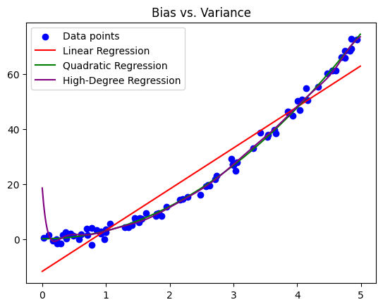
In the above case, the purple line represents a model with high variance (degree=15), capturing even more intricate details in the training data. While it fits the training data well, it is likely to perform poorly on new data due to overfitting.

The goal is to find the right balance between bias and variance, avoiding both underfitting and overfitting. This is often achieved through techniques like cross-validation, regularization, and careful feature selection.

Understanding and addressing overfitting, underfitting, bias, and variance are crucial steps in building robust and generalizable machine learning models.

Let's go through simple examples for each concept.

import numpy as np
import matplotlib.pyplot as plt

# Generate some noisy sine wave data
np.random.seed(42)
X = np.sort(5 * np.random.rand(80, 1), axis=0)
y = np.sin(X).ravel() + np.random.normal(0, 0.1, X.shape[0])

# Fit a high-degree polynomial
degree = 15
coefficients = np.polyfit(X.ravel(), y, degree)
poly = np.poly1d(coefficients)

# Plot the data and the overfitting model
plt.scatter(X, y, color='blue', label='Data points')
x_range = np.linspace(0, 5, 100)
plt.plot(x_range, poly(x_range), color='red', label=f'Overfitting (Degree {degree})')
plt.title('Overfitting Example')
plt.legend()
plt.show()

Output

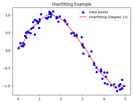
In the above example, fitting a high-degree polynomial to a simple sine wave introduces overfitting. The model memorizes the noise in the training data, capturing more details than necessary.

import numpy as np
import matplotlib.pyplot as plt

# Generate some linear data
np.random.seed(42)
X = 5 * np.random.rand(80, 1)
y = 2 * X + 1 + np.random.randn(80, 1)

# Fit a linear model to quadratic data
from sklearn.linear_model import LinearRegression
from sklearn.preprocessing import PolynomialFeatures
from sklearn.pipeline import make_pipeline

model = make_pipeline(PolynomialFeatures(1), LinearRegression())
model.fit(X, y)

# Plot the data and the underfitting model
plt.scatter(X, y, color='blue', label='Data points')
plt.plot(X, model.predict(X), color='red', label='Underfitting (Linear Model)')
plt.title('Underfitting Example')
plt.legend()
plt.show()

Output

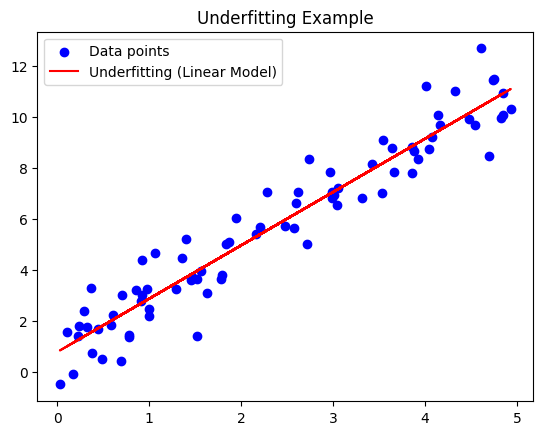
In the above example, fitting a linear model to quadratic data results in underfitting. The model is too simple to capture the underlying quadratic pattern.

import numpy as np
import matplotlib.pyplot as plt

# Generate some data with a linear relationship
np.random.seed(42)
X = 2 * np.random.rand(100, 1)
y = 4 + 3 * X + np.random.randn(100, 1)

# Fit a linear model with a bias
from sklearn.linear_model import LinearRegression

model = LinearRegression(fit_intercept=True)
model.fit(X, y)

# Plot the data and the biased model
plt.scatter(X, y, color='blue', label='Data points')
plt.plot(X, model.predict(X), color='red', label='Biased Model')
plt.title('Bias Example')
plt.legend()
plt.show()

Output

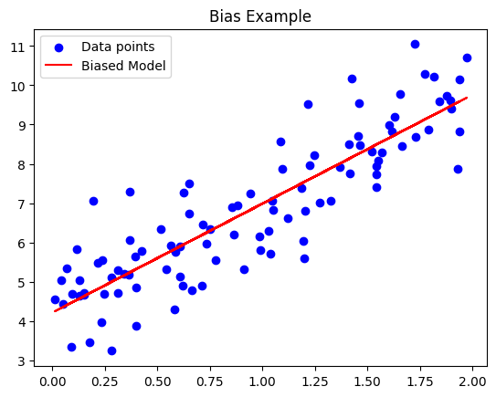
In the above example, the model has a consistent bias (intercept) in the positive direction, consistently making mistakes by predicting values higher than the true values.

import numpy as np
import matplotlib.pyplot as plt

# Generate some data with a linear relationship
np.random.seed(42)
X = 2 * np.random.rand(100, 1)
y = 4 + 3 * X + np.random.randn(100, 1)

# Fit a high-variance model
from sklearn.tree import DecisionTreeRegressor

model = DecisionTreeRegressor(max_depth=10)
model.fit(X, y)

# Plot the data and the high-variance model
plt.scatter(X, y, color='blue', label='Data points')
x_range = np.linspace(0, 2, 100).reshape(-1, 1)
plt.plot(x_range, model.predict(x_range), color='red', label='High-Variance Model')
plt.title('Variance Example')
plt.legend()
plt.show()

Output

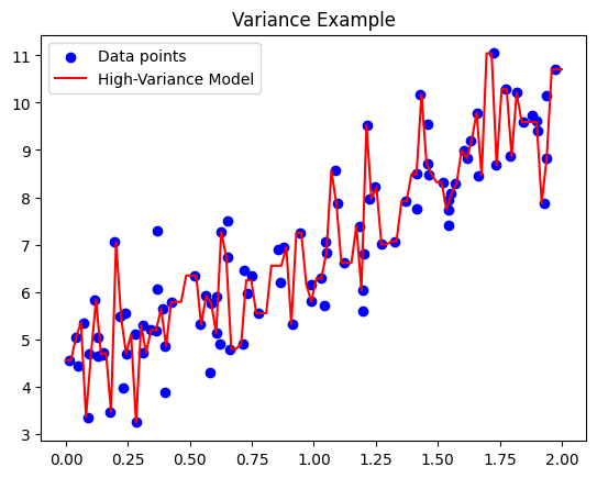
In the above example, the decision tree model is highly sensitive to small changes in the data, capturing the noise and fluctuations, leading to high variance.

In conclusion, mastering the delicate interplay of overfitting, underfitting, bias, and variance is the key to building robust and effective machine learning models. Recognizing the pitfalls of overfitting and underfitting allows data scientists to navigate the complexity of real-world problems successfully. While overfitting tempts the model to memorize the nuances of the training data, underfitting oversimplifies the learning process, leading to suboptimal performance.

Understanding bias and variance provides a lens through which to view a model's consistency and sensitivity. High bias manifests as unwavering mistakes, akin to a model with a narrow worldview. Meanwhile, high variance turns a model into a chameleon, adapting to every idiosyncrasy of the training data but failing to generalize. As data scientists navigate this landscape, the mastery of overfitting, underfitting, bias, and variance becomes a powerful compass, guiding them toward models that stand resilient in the face of diverse and unpredictable data.