[Do you already know what MaxDiff is, and can you find your way around in R? You could skip to the end and find a big code block with everything you need.]

MaxDiff is the combination of a survey method and statistical estimation process to determine preferences for items on a list. It is becoming widely used to prioritize product features, use cases, consumer preferences, employee benefits, advertising messages, public policy positions, and many other topics.

The general concept of MaxDiff is to prioritize a long list more reliably than other methods. A long list is difficult to stack rank reliably by an individual, and the resulting ordinal rankings are not as useful as interval-scale rankings. Other alternatives such as Likert grid ratings tend to to say "everything is important."

Here's an example from Chapter 10 of the Quant UX Book. If I ran a pizza restaurant, I might survey customers about pizza preferences using a grid item, such as:

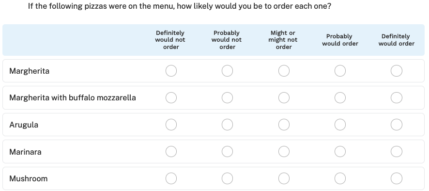
But that doesn't tell us much. Suppose the average for Mushroom pizza is "probably would order." How many pizzas would I expect to sell? How much more likely is someone to order a mushroom pizza vs. a Marinara pizza? There is no way to know. MaxDiff gives a better answer by presenting a forced-choice item that more closely mimics a real-world choice situation:

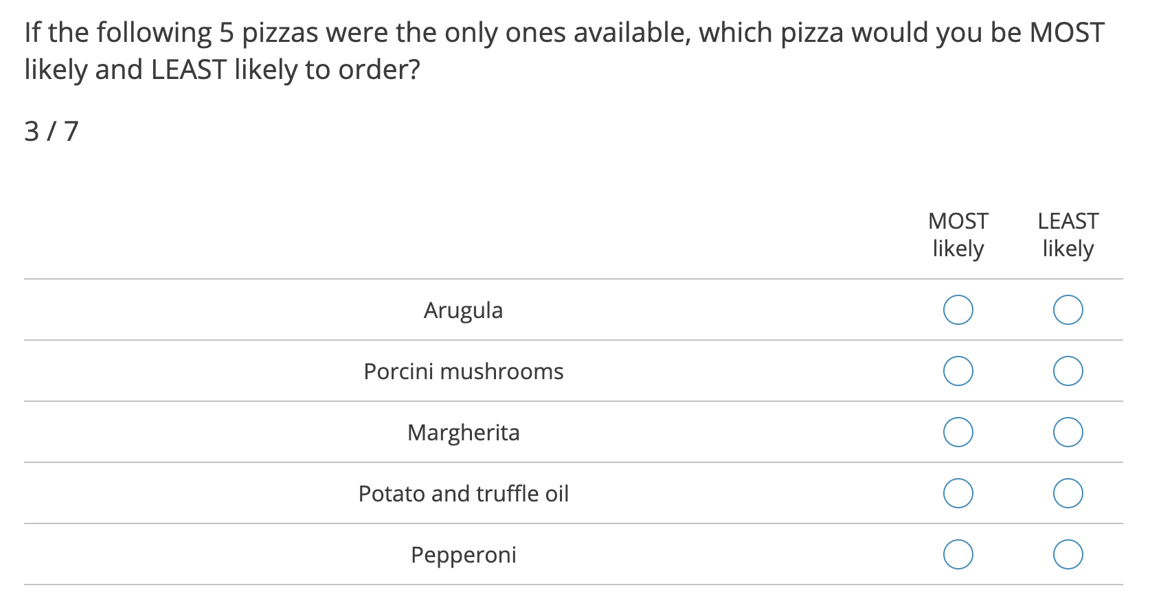
The results give choice likelihood in the presence of trade-offs. In the Quant UX Book, Kerry Rodden and I demonstrate MaxDiff for pizza preference and then for product use case importance. But that chapter relies on a complex set of dependencies: Qualtrics or another survey platform, plus advanced R code.

In this post, I demonstrate MaxDiff in base R alone (plus the ggplot2 package). I have a few goals:

Make it easy to see how MaxDiff works. All you need is this code and R.
Make Chapter 10 of the Quant UX book more approachable. (Not that I believe it is unapproachable now, although it is the most complex in the book!)
Let you use MaxDiff for yourself. I often use MaxDiff to prioritize personal things. This code will let you do that without setting up a survey or complex code. As we'll see, MaxDiff works pretty well even with N=1. (True story: Kerry and I used MaxDiff with N=2 to compare our goals in writing the Quant UX book.)

This code is not intended for user data collection, because you wouldn't sit users down at an R console (I hope!) Instead, it's a fast demo of MaxDiff.

You don't need to know very much R to use it, just enough to edit the items and run a few lines of code. (OTOH, I hope it might encourage you to learn more R.)

Similar to my other R posts, I'll walk through and explain the code. You can find the entire code file for copy-and-paste purposes at the end of this post.

Step 1: Set Up the Questions and Responses

There are two preliminary setup steps:

If you don't have them already, install R and RStudio, then run RStudio and install the ggplot2 package (command install.packages("ggplot2")). (TBH, if you don't already have those, then this post may not be for you.)
Copy/paste the entire code file from the end of this post into a new script file in RStudio. Then "source" the code inside RStudio using the Source button at the upper right of the editor. That adds the MaxDiff functions to your workspace.

Here's the problem we'll solve in this post. In the book, I showed how to find and then the results of my personal pizza preferences. Now I'll prioritize ice cream preferences. We'll see how to do that, from setting up the question and items, through collecting data, to seeing the result.

The code starts by initializing a new study object, which will hold the MaxDiff items and any data. I'll call that object mdIce, which is a list to hold everything else.

# initialize study and set up items
mdIce            <- init_study()

If you get an error such as Error in init_study() : could not find function "init_study" then you likely need to copy/paste and source the code file, as described above, and described in the code block at the end of this post. Sourcing it into your R session makes the functions available.

Next, we add 13 flavors of ice cream to the study. See Chapter 10 in the Quant UX Book for discussions about how many items to use, sample size requirements, etc.

In this case, I add the Items (13 flavors) that I want to prioritize into the study object:

mdIce$Items      <- c("Chocolate", "Vanilla", "Strawberry", "Espresso", 
                      "Pistachio", "Orange Sherbet", "No Fat Vanilla Yogurt", 
                      "Caramel", "Chocolate Chip", "Mint Chocolate Chip", 
                      "Lemon Sherbet", "Rocky Road", "Brownie Bites")

(Side note. I'll admit some of those are not "ice cream." As you'll see, I also don't like them! More seriously, this gets to the point of writing items that users understand.)

MaxDiff item texts are sometimes very long. For plotting you may want to use shorter text. We set up ShortItems next, which become the "friendly names" used in the data set and on charts. I'll shorten one of the flavor descriptions:

mdIce$ShortItems <- mdIce$Items                                                  # short names for chart
mdIce$ShortItems[mdIce$ShortItems=="No Fat Vanilla Yogurt"] <- "No Fat Vanilla"  # shorten one item

We complete the setup by writing the question headers that will be presented — the bestQuestion and worstQuestion — and tell the code the number of items to show in each response set. In this case, I'll show 6 ice cream flavors at a time. (For more complex tasks, you would want to show fewer, perhaps 3, 4, or 5 items at a time. We discuss that in the book chapter.)

# set up the questions
mdIce$bestQuestion  <- "Among these ice cream flavors, which one do you like MOST? (enter the line number)"
mdIce$worstQuestion <- gsub("MOST", "LEAST", mdIce$bestQuestion)
mdIce$numItems      <- 6

In this case, each response will ask the respondent to choose the most and least preferred ice cream flavor from a set of 6 flavors at a time, drawn randomly from the longer list of 13.

The study is now ready to collect data! That was 7 lines of R code (depending on how you count them). Wasn't that easier than writing a survey using a survey platform?

Step 2: Collect Responses

This code collects responses interactively in the R console (aka command line, aka terminal) window. Run the add_choices() function to begin; be sure to save its result, as in the code. Answer as many as you wish, and enter "0" to stop.

# collect the data in R console
mdIce <- add_choices(mdIce)            # can run this on a new study, or an existing one to add data

Look at your R console window and enter choices, as in this screenshot:

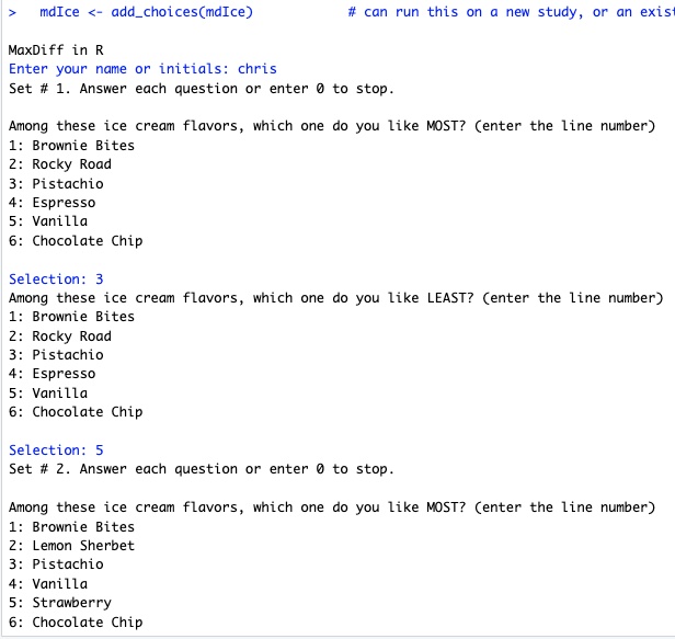
In this series of choices, I said that Pistachio was the best and Vanilla was the worst, among the first 6 flavors. Then it went to a new set. After answering 20 sets, I entered "0" to stop.

Yes, 20 is a lot of choices but you can make as few or as many responses as you wish, and it will work with the data it has. OTOH, after the first couple of sets, MaxDiff goes very quickly, both in this case and with real respondent data.

BTW, you can always run add_choices() again to gather more data. Try adding some random responses, too!

Step 3: See the Results

This code uses the "counts" method for MaxDiff scoring, which is simple and easy to explain (see Next Steps below for other options). It counts how often an item was chosen as best, and how often it was chosen as worst, relative to how many times it was shown. The net preference is the difference between those two relative counts.

The code for that is:

find_counts(mdIce)                     # data frame with the counts

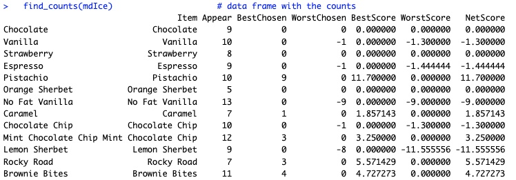
Below are the results for my ice cream preferences. Here's how the simple scoring works. Among the choice sets, Pistachio appeared 10 times and among those, I chose it as the best flavor in 9 sets.

Yet each set is chosen randomly, so the possible chances to win or lose vary across items. If Pistachio had appeared as often as the most-often-appearing flavor (No Fat Vanilla) it would have appeared 13 times. (Side note: survey platforms such as Sawtooth Software determine an efficient and balanced design matrix to avoid this issue.)

To correct for the chances to win, Pistachio's score is adjusted to match the relative number of appearances: 9 chosen * 13 max appearances / 10 actual appearances = 11.70 as its final score for being chosen best. (It was never chosen as worst, so that is also its final net score. Otherwise, the same adjustment is carried out on the "worst" side of the score.)

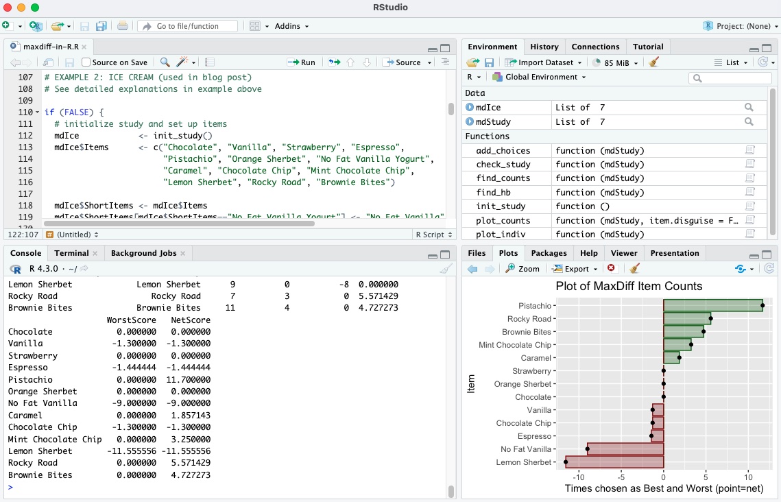
You can see that Pistachio was my favorite among these, while Lemon Sherbet was the least preferred. I was indifferent to chocolate, strawberry, and some others, which were rarely or never chosen as best or worst.

This is all much easier to see on a chart! The plot_counts() function does that:

plot_counts(mdIce)                     # ggplot2 plot of the counts and net counts

Here's the result:

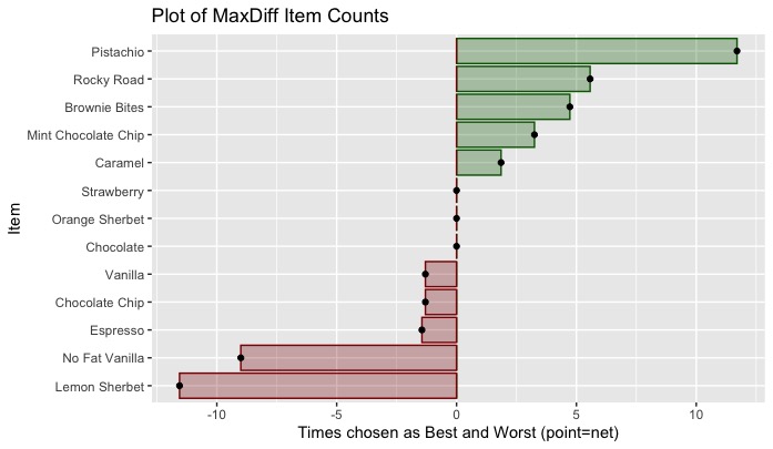
In this case, I had no items that were sometimes best but also sometimes worst, so the net scores (shown as points) are identical to the best or worst scores (shown as bars). After more selections — or adding some random responses — that would be likely to change.

If I'm in Rome and get gelato after pizza, now you know what I'm most likely to order!

Next Steps

As you saw, MaxDiff is pretty easy and is mostly about writing a good set of items. In this post, it took us only a total of 10 lines of R: 7 lines to set up the study, 1 line to collect data, and 2 line to see and chart the results. To be fair, this is a simple demo and not adequate for important research ... but it can get you started with MaxDiff!

Here are some suggestions on next steps:

Adapt the code to something you would like to prioritize and try it out! Some suggested things to prioritize for yourself include:
1. Food or beverage preferences
2. Places to go on vacation
3. Baby or pet names
4. Amenities of importance when buying or renting a home
5. Team morale or off-site events
6. Features that matter to you when job-searching
7. Favorite books, music, or movies
8. ... and of course work-related things, like use cases and product features
I didn't describe it above, but the code includes one bonus feature: if you collect responses with two or more names/initials, the functions find_counts_indiv(mdStudy) and plot_counts_indiv(mdStudy) will compare their scores. (Replace mdStudy with the name of your study object, such as mdIce in the example above.)
If you'd like to learn more about MaxDiff — writing the items, designing a survey, using it for real user situations, and estimating results — see Chapter 10 in the Quant UX book. That chapter covers everything you need to know to get started with larger, important projects.
The first part of a real application is to select a survey platform that supports the MaxDiff response type (selecting a subset of items, and collecting "best" and "worst" among each set). The most comprehensive option is Sawtooth Software's Lighthouse Studio, while Qualtrics, Conjoint.ly, and other platforms have varying degrees of support.
The second part of a real application is to estimate the preference statistics. The counts model used here is the simplest and it works pretty well. Better, however, is a hierarchical Bayes (HB) model that finds individuals' preferences nested within a group distribution. Chapter 10 of the Quant UX Book demonstrates HB for MaxDiff, while Chapters 9 and 13 of the R book explain more about HB models and discrete choice surveys (of which MaxDiff is one variation).
Although powerful, MaxDiff is not magical. Be sure to pre-test any surveys with live users, and review other concerns in the Quant UX Book. Or read a dedicated book such as Chrzan and Orme (2019), Applied MaxDiff.

I hope this made MaxDiff easier for you!

Entire code chunk for copy-and-paste

Create a new R script file in RStudio. Then click on the "copy" icon on the upper right of the code box below, and paste it into that file.
Source that file inside RStudio using the "Source" button (upper right hand in the editor window). That adds the functions to your workspace.
Read the code up to line 47, and then adapt it to your own problem or example.

# Interactive MaxDiff in R
#
# Version: 0.1
# October 6, 2023
#
# ==> A demonstration of MaxDiff for single users (or a few people who can share one machine)
# ==> TO GET STARTED: Skip down to line 47 unless you like fine print
#
# Author:  Chris Chapman
# Follow:  quantuxblog.com  |  https://www.linkedin.com/in/cnchapman/ 
#
# Rights:  (c) Chris Chapman, 2023. Rights reserved as noted in the license.
#
# License: Shared openly under the CC BY-NC-SA 4.0 License, which means you may 
#          "distribute, remix, adapt, and build upon the material in any medium or 
#          format for noncommercial purposes only, and only so long as attribution 
#          is given to the creator. If you remix, adapt, or build upon the material, 
#          you must license the modified material under identical terms."
#          https://creativecommons.org/licenses/by-nc-sa/4.0/
# 

########################################
# GENERAL DESCRIPTION
# Code that can be used by one person to demonstrate MaxDiff for themselves,
# using nothing more than the R console. It computes simple best-worst counts, 
# which are very highly correlated (e.g., typically r > 0.9) with more advanced
# estimation.
# 
# This will let you see how MaxDiff works, and also use it for personal projects
# (such as prioritizing goals) without the overhead of using a survey platform.

########################################
# HOW TO USE: DESCRIPTIVE (but see the EXAMPLE below for a walkthrough)
#
# 1. Brainstorm the question you want to ask and the list of items to be sorted
#    (see Chapter 10 in Chapman & Rodden, 2023, Quantitative User Experience Research)
#
# 2. Set up an mdStudy object as demonstrated below, using the init_study() function.
#    This mdStudy object will hold your items, questions, and collected data
#
# 3. Gather responses interactively in the R console, using the add_choices() function
#    and put those back into the mdStudy object (or somewhere else that you prefer)
#
# 4. See the results using find_counts(mdStudy) and plot_counts(mdStudy)

########################################
# HOW TO USE: EXAMPLE CODE
#
# 1. If needed, install the "ggplot2" package; it is the only dependency for basic usage.
# 2. Source() this file (in RStudio, click "Source" at the upper right hand of the editor window).
#    That will add the functions that you need to your global workspace (no need for a package).
# 3. Run each line of code inside the FALSE block below for an interactive example.
# 
#   NOTES ON THE EXAMPLE: 
#   The following example is set up to find the "best" and "worst" among first 12 English letters.
#   You could answer in any way you prefer; for example, that "A" is best and higher letters are worse.
#   It's helpful to have an answering strategy so you can see how the plots and counts work.
#   It's also helpful to add noise and random responses, to see how those affect it.
#   After collecting a few responses, try plotting it; then run add_study() again to collect more.
#
# TRY IT !
#
if (FALSE) {                    # run each statement inside this block, one by one, to see how it works
  #####
  ##### Set up everything
  ##### 
  # initialize a study object
  mdStudy <- init_study()

  # set up our items
  # we will use letters of the English alphabet as prompts
  mdStudy$Items      <- LETTERS[1:12]   # long-form text that respondents would see for each item
  mdStudy$ShortItems <- LETTERS[1:12]   # short "friendly names" that will be plotted and used for column names

  # set up the question headers that will be asked
  mdStudy$bestQuestion <- "Among these letters, which one do you like MOST? (enter the line number)"
  mdStudy$worstQuestion <- gsub("MOST", "LEAST", mdStudy$bestQuestion)

  # set up how many items to ask at any given time (should be 2-8, most commonly 4 or 5 at a time)
  mdStudy$numItems <- 4

  #####
  ##### Collect some data in the R console
  #####
  # collect the data in R console [ look at the console after running! ]
  mdStudy <- add_choices(mdStudy)          # can run this on a new study, or an existing one to add data

  # compute simple count scores
  find_counts(mdStudy)                     # data frame with the counts

  # plot the results
  plot_counts(mdStudy)                     # ggplot2 plot of the counts and net counts

  # ... and then go back to the "add_choices()" statement a few lines above, and collect more data
  # ... repeat as desired

  # THAT'S IT!

  # NEXT STEPS:
  # create a new mdStudy object
  # set up its Items, ShortItems, and Questions for a problem you care about
  # collect data from yourself for your problem, and see your preferences
}


########################################
# EXAMPLE 2: ICE CREAM (used in blog post)
# See detailed explanations in example above

if (FALSE) {                    
  # initialize study and set up items
  mdIce            <- init_study()
  mdIce$Items      <- c("Chocolate", "Vanilla", "Strawberry", "Espresso", 
                        "Pistachio", "Orange Sherbet", "No Fat Vanilla Yogurt", 
                        "Caramel", "Chocolate Chip", "Mint Chocolate Chip", 
                        "Lemon Sherbet", "Rocky Road", "Brownie Bites")

  mdIce$ShortItems <- mdIce$Items                                                  # short names for chart
  mdIce$ShortItems[mdIce$ShortItems=="No Fat Vanilla Yogurt"] <- "No Fat Vanilla"  # shorten one item

  # set up the questions
  mdIce$bestQuestion  <- "Among these ice cream flavors, which one do you like MOST? (enter the line number)"
  mdIce$worstQuestion <- gsub("MOST", "LEAST", mdIce$bestQuestion)
  mdIce$numItems      <- 6

  # collect the data in R console
  mdIce <- add_choices(mdIce)            # can run this on a new study, or an existing one to add data

  # get scores and plot
  find_counts(mdIce)                     # data frame with the counts
  plot_counts(mdIce)                     # ggplot2 plot of the counts and net counts
}


### END OF DIDACTIC CODE AND DEMONSTRATION
########################################



########################################
# FUNCTIONS
# Generally DO NOT CHANGE anything below this line
#
# ... unless, of course, you're learning or adapting it per the license permissions
#


########################################
# INITIALIZATION FUNCTION

# initializes a dummy study with all the slots needed to hold items and data
# replace the items and item friendly names with the data you need, as 
# shown in the examples above
#
init_study <- function() {
  mdStudy <- list(
    # The text of the items that you want to ask, one item per row.
    # must have at least as many as the "numItems" setting below, and
    # typically somewhere between 10 to 30 items
    #
    # WARNING: do not add or delete items, nor substantially edit them 
    #          after collecting observations. You may collect more 
    #          observations, but if you edit the *items* then the collected
    #          data might not make sense (and/or the scripts may fail)
    #
    Items = c(
      "item 1",
      "item 2",
      "item 3",
      "item 4",
      "item 5",
      "item 6",
      "item 7",
      "item 8",
      "item 9",
      "item 10",
      "item 11",
      "item 12"
    ),

    # set shorter "friendly names" to use in data frames and charts instead of 
    # the user-shown item texts above
    ShortItems = paste0("i", 1:12),

    # how many choices to present in one set (drawn randomly from Items above)
    numItems = 4,

    # prompts for the two MaxDiff questions asked about each set of items
    bestQuestion  = "MOST ... Which of these do you prefer MOST ?",
    worstQuestion = "LEAST ... Which of these do you prefer LEAST ?",

    # places to store the observations and other metadata
    Observations = NULL,
    Count = NULL
  )
  return(mdStudy)
}

########################################
# DATA COLLECTION FUNCTIONS

# check_study()
#   do some basic data validation on the study design
#   and return appropriate warning for any detected problems
#   ... TBW

check_study <- function(mdStudy) {
  studyCheck <- "OK"
  # check that observations are null, if count is null
  if (is.null(mdStudy$Count) != is.null(mdStudy$Observations)) {
    studyCheck <- "The study observations and count do not match; only one of them is NULL. Check your mdStudy object."
  }
  # check that any observations match the short items' length & names
  if (!is.null(mdStudy$Observations)) {
    if (ncol(mdStudy$Observations) != (length(mdStudy$ShortItems)+5)) {
      studyCheck <- "Columns in mdStudy$Observations do not match expectation based on mdStudy$ShortItems."
    }
  }
  # check length items == length short items
  if (length(mdStudy$Items) != length(mdStudy$ShortItems)) {
    studyCheck <- "In the mdStudy object, Items and ShortItems have unequal lengths."
  }
  # check numitems is reasonable (2-8, and also <= number of items)
  if (mdStudy$numItems < 2) {
    studyCheck <- "Cannot do a MaxDiff task with fewer than 2 items. Check mdStudy$numItems."
  } 
  if (mdStudy$numItems >= length(mdStudy$Items)) {
    studyCheck <- "You have too many items per tasks (mdStudy$numItems) relative to the total items ($Items)."
  }
  if (mdStudy$numItems > 8) {
    studyCheck <- "You have more than 8 items per task (mdStudy$numItems) which is likely too difficult."
  }
  return(studyCheck)
}


# add_choices()
#   collect responses from user in the R console

add_choices <- function(mdStudy) {
  # make a copy that we'll modify and return
  mdResult <- mdStudy

  #####
  # FIRST make sure a few things are set up OK and give a warning if not
  check <- check_study(mdResult)
  if (check != "OK") {
    cat("The following error was found. Will continue, but you should probably stop and fix this.\n")
    cat(check)
  }

  #####
  # NOW collect the data
  # get respondent name
  cat("\nMaxDiff in R\n")
  respName <- readline("Enter your name or initials: ")

  # get respondent's observations
  continue  <- TRUE
  taskcount <- ifelse(is.null(mdResult$Count), 0, mdResult$Count)
  while (continue) {
    taskcount <- taskcount + 1
    cat(paste0("Set # ", taskcount, ". Answer each question or enter 0 to stop.\n\n"))

    # sample the items to show
    itemCols <- sample(length(mdResult$Items), mdResult$numItems)
    items    <- mdResult$Items[itemCols]

    # show B & W items and get input
    cat(mdResult$bestQuestion)
    bestAnswer <- menu(items)

    if (bestAnswer > 0) {
      cat(mdResult$worstQuestion)
      worstAnswer <- menu(items)
    }

    # check and save observation
    # if input == stop then continue <- FALSE 
    if (bestAnswer==0 || worstAnswer==0) {
      continue <- FALSE
    } else {
      # set up this single block observation
      # using the "md.block" format from choicetools package
      oneObs <- data.frame(matrix(0, nrow=mdResult$numItems*2, ncol=length(mdResult$ShortItems)+5))
      names(oneObs) <- c("win", "resp.id", 
                         mdResult$ShortItems,
                         "Block", "Set", "sys.resp")
      # metadata
      oneObs$resp.id  <- respName   # used as respondent identified in hierarchical models
      oneObs$sys.resp <- respName   # carry-over from Sawtooth Software related legacy code
      oneObs$Set      <- rep(c("Best", "Worst"), each=mdResult$numItems)
      oneObs$Block    <- taskcount
      # design matrix
      for (i in seq_along(itemCols)) {
        oneObs[i, itemCols[i]+2]                     <-  1     # Best design matrix entry for sampled item i
        oneObs[i + mdResult$numItems, itemCols[i]+2] <- -1     # Worst design matrix entry for sampled item i
      }
      # choices
      oneObs[bestAnswer, "win"]                      <- 1
      oneObs[worstAnswer + mdResult$numItems, "win"] <- 1

      # add the block to the overall set of data
      mdResult$Observations <- rbind(mdResult$Observations, oneObs)
      mdResult$Count        <- taskcount
    }
  }
  return(mdResult)
}


########################################
# RESULTS FUNCTIONS

# plot_counts()
#   plot simple best | worst | best-worst chart for the responses
# 
#   this plot adjusts each count according to the relative number of times each item was shown
#   so that random variations in the number of times that items appear in small-N data do not
#   drown out the best/worst signal

plot_counts <- function(mdStudy, item.disguise=FALSE) {

  # the following is adapted from Chapman et al, "choicetools" package
  # https://github.com/cnchapman/choicetools
  # 
  plot.md.counts <- function(md.define, item.disguise=FALSE) {
    if (is.null(md.define$md.block)) {
      stop("Could not find md.block matrix within the md.define object. Make sure data have been loaded first.")
    }
    exclude.cols <- c("win", "resp.id", "Block", "sys.resp", "Set", "choice.coded")
    item.cols    <- names(md.define$md.block)
    item.cols    <- item.cols[!item.cols %in% exclude.cols]

    best.appear <- colSums(md.define$md.block[md.define$md.block$Set=="Best", item.cols])
    best.win    <- colSums(md.define$md.block[md.define$md.block$Set=="Best" &
                                                md.define$md.block$win==1, item.cols])

    worst.appear <- colSums(md.define$md.block[md.define$md.block$Set=="Worst", item.cols])
    worst.win    <- colSums(md.define$md.block[md.define$md.block$Set=="Worst" &
                                                 md.define$md.block$win==1, item.cols])

    item.scale  <- max(best.appear) / best.appear

    md.counts <- data.frame(Item  = item.cols,
                            Best  = best.win*item.scale,
                            Worst = worst.win*item.scale)

    if (item.disguise) {
      md.counts$Item <- paste0("i", 1:nrow(md.counts))
    }

    library(ggplot2)
    p <- ggplot(aes(x=reorder(Item, Best+Worst), y=Best),
                data=md.counts) +
      geom_col(alpha=0.3, color="darkgreen", fill="darkgreen") +
      geom_col(aes(x=Item, y=Worst), alpha=0.3, color="darkred", fill="darkred") +
      geom_point(aes(x=Item, y=Best+Worst), color="black", shape=19, size=1.5) +
      coord_flip() +
      ggtitle("Plot of MaxDiff Item Counts") +
      ylab("Times chosen as Best and Worst (point=net)") +
      xlab(ifelse(item.disguise, "Item (Disguised)", "Item"))
    p
  }

  # munge mdStudy into the choicetools format so we can use the plot function
  md.define <- list()
  md.define$md.block <- mdStudy$Observations

  # make the plot and return it
  p <- plot.md.counts(md.define, item.disguise = item.disguise)
  return(p)
}

# find_counts()
#   compute simple best | worst | best-worst chart for the responses
# 
#   this function adjusts each count according to the relative number of times each item was shown
#   so that random variations in the number of times that items appear in small-N data do not
#   drown out the best/worst signal

find_counts <- function(mdStudy) {
  exclude.cols <- c("win", "resp.id", "Block", "sys.resp", "Set")
  item.cols    <- names(mdStudy$Observations)
  item.cols    <- item.cols[!item.cols %in% exclude.cols]

  best.appear <- colSums(mdStudy$Observations[mdStudy$Observations$Set=="Best", item.cols])
  best.win    <- colSums(mdStudy$Observations[mdStudy$Observations$Set=="Best" &
                                                mdStudy$Observations$win==1, item.cols])

  worst.appear <- colSums(mdStudy$Observations[mdStudy$Observations$Set=="Worst", item.cols])
  worst.win    <- colSums(mdStudy$Observations[mdStudy$Observations$Set=="Worst" &
                                                 mdStudy$Observations$win==1, item.cols])

  item.scale  <- max(best.appear) / best.appear

  md.counts <- data.frame(Item  = item.cols,
                          Appear      = best.appear,
                          BestChosen  = best.win,
                          WorstChosen = worst.win,
                          BestScore   = best.win*item.scale,
                          WorstScore  = worst.win*item.scale,
                          NetScore    = best.win*item.scale + worst.win*item.scale)

  return(md.counts)
}

# find_counts_indiv()
#   find net score for each unique respondent ID in a study object
# 
#   runs find_counts() for each group of data by resp.id as collected in console responses
#   and returns the result as a data frame

find_counts_indiv  <- function(mdStudy) {
  # make sure there are observations
  if (is.null(mdStudy$Observations)) {
    stop("The study object does not have observed data.")
  }
  # get net scores for each individual ID
  counts.inds <- NULL
  unique.ids  <- unique(mdStudy$Observations$resp.id)

  if (length(unique.ids) == 0) {
    warning("Could not find respondent IDs in the study observations.")
  } else {
    for (i in unique.ids) {
      tmpStudy <- mdStudy
      tmpStudy$Observations <- subset(tmpStudy$Observations, resp.id==i)
      tmpCounts   <- find_counts(tmpStudy)
      counts.one  <- data.frame(Name=i, Item=tmpCounts$Item, `Net Score`=tmpCounts$NetScore)
      counts.inds <- rbind(counts.inds, counts.one)
    }
  }
  counts.inds$Name <- factor(counts.inds$Name)
  return(counts.inds)
}


# plot_counts_indiv()
#   plots the net score by item for each unique respondent
# 
#   runs find_counts_indiv() and plots the result
#   this is most useful to compare a moderate number of respondents
#   note that the return object is a ggplot2 object, if you'd like to tinker
#   with axis or chart titles, alpha levels, coordinate limits, etc.

plot_counts_indiv <- function(mdStudy) {
  counts.ind <- find_counts_indiv(mdStudy)
  library(ggplot2)
  p <- ggplot(counts.ind, aes(x=Item, y=Net.Score, group=Name, color=Name)) +
    geom_line(alpha=0.3) +
    geom_point() +
    ylab("Net Score") +
    coord_flip()
  return(p)
}

Easy MaxDiff in R