Peach crop plants are susceptible to several diseases, which can have a significant impact on yield. Early detection and diagnosis of these diseases are essential for effective control measures to be implemented.

Traditional methods of disease detection are time-consuming and require expertise, which can be limited in some areas. Machine learning (ML) offers a promising alternative, with the potential to automate disease detection and make it more accessible to farmers.

Tensorflow is a good choice for binary classification problems, such as classifying peach crop plants as infected or healthy. It provides several features that make it well-suited for this task.

CNN Model for Peach Crop Plant Classification

Convolutional neural networks (CNNs) are effective for a variety of image classification tasks, including peach crop classification. CNNs can learn complex features from images that can be used to distinguish between different classes.

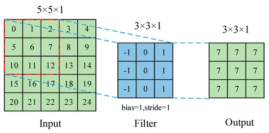
Process of Convolution Operation :

Process of Pooling Operation :

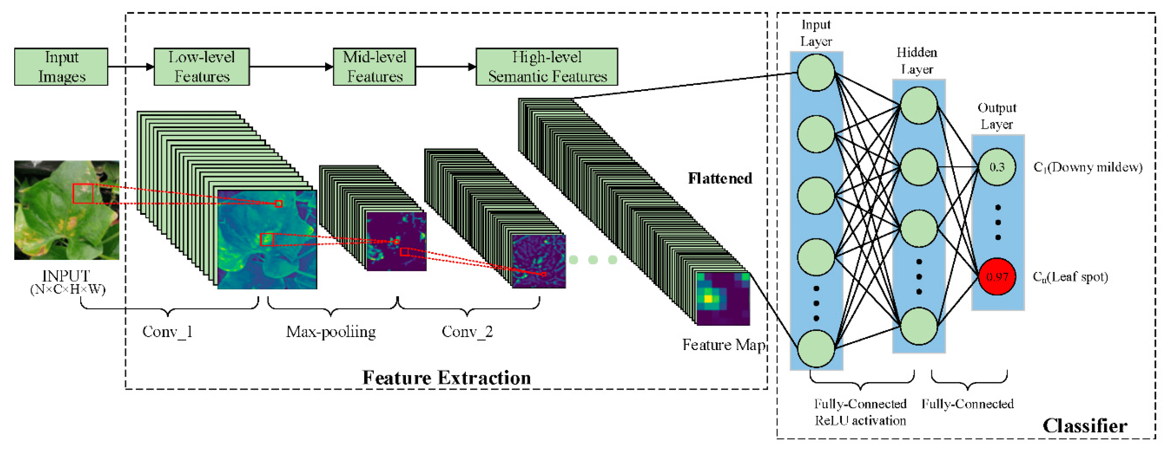
Overall Process :

Let us build a model using Tensorflow CNN that will classify the crop to be healthy or infected by taking the image of the leaf of the peach crop plant. For that, you would need to collect a dataset of images of infected and healthy plants. The images were downloaded from Kaggle Peach Crop Village Ds. There are 2656 images of leaves (infected and healthy) of peach crop plants.

Let us train our Convolutional Neural Network.

Import Libraries

import tensorflow as tf
from tensorflow.keras.preprocessing.image import ImageDataGenerator
from tensorflow.keras import Sequential
from tensorflow.keras.layers import Conv2D,MaxPooling2D,Flatten,Dense
import matplotlib.pyplot as plt

Loading Images

To load the images from the dataset, We will use the ImageDatagenerator module from tensorflow.keras.preprocessing.image with which we can directly load the images by rescaling the pixel values of the images between '0 and 1'( rescale = 1/255.0 ) which decreases computational complexity. And also split the data into train and test directly ( validation_split = 0.2 ), which is useful for testing the performance of the model on unseen data.

Also, The ImageDataGenerator class allows you to augment your image data by applying random transformations to the images, such as rotations, flips, and zooms. Which is a powerful technique that can be used to improve the performance of machine learning models on a variety of tasks.

Data Augmentation

rotation_range: This parameter controls the range of random rotations that will be applied to the images. For example, if you set rotation_range=90, then the images will be randomly rotated by up to 90 degrees in either direction.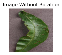
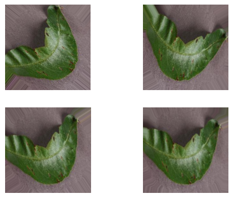
images with rotation_range=90 applied.
width_shift_range: This parameter controls the range of random horizontal shifts that will be applied to the images. For example, if you set width_shift_range=0.2, then the images will be randomly shifted horizontally by up to 20% of their width in either direction.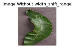
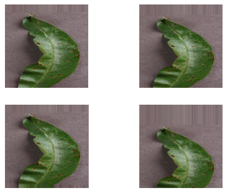
images with width_shift_range=0.2 applied.
height_shift_range: This parameter controls the range of random vertical shifts that will be applied to the images. For example, if you set height_shift_range=0.2, then the images will be randomly shifted vertically by up to 20% of their height in either direction.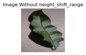
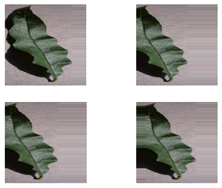
images with height_shift_range=0.2 applied.
shear_range: This parameter controls the range of random shear transformations that will be applied to the images. A shear transformation is a transformation that slants the image horizontally or vertically. For example, if you set shear_range=0.2, then the images will be randomly sheared by up to 20 degrees in either direction.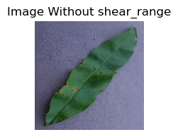
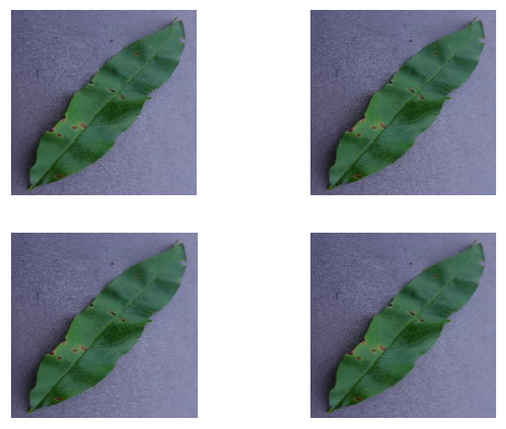
images with shear_range=0.2 applied.
zoom_range: This parameter controls the range of random zoom transformations that will be applied to the images. For example, if you set zoom_range=0.4, then the images will be randomly zoomed in or out by up to 40% of their original size.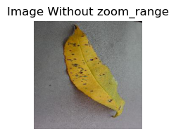
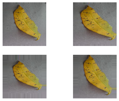
images with zoom_range=0.4 applied.
horizontal_flip: This parameter controls whether to randomly flip the images horizontally. This can be a useful augmentation technique for images that are invariant to horizontal flips, such as images of cars or aeroplanes.
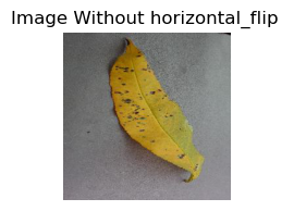
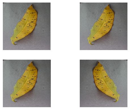
images with horizantal_flip applied.
fill_mode: This parameter controls the mode used to fill in pixels that are outside of the image boundary after a transformation. The valid options are nearest, constant, reflect, and wrap.
The nearest fill mode simply copies the nearest pixel to the boundary. The constant fill mode fills in the boundary with a constant value. The reflect fill mode reflects the image across the boundary. The wrap fill mode wraps the image around the boundary.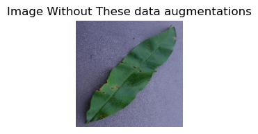
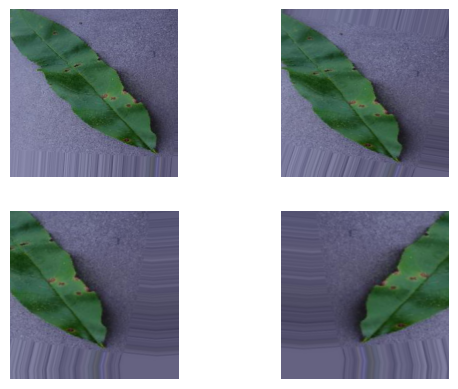
You can experiment with different augmentation parameters to find what works best for your dataset and model. It is generally recommended to use a variety of augmentation techniques to improve the performance of your model☺️.

datagen = ImageDataGenerator(
    rescale = 1/255.0,
    rotation_range = 40, 
    width_shift_range = 0.2, 
    height_shift_range = 0.2, 
    shear_range = 0.2, 
    zoom_range = 0.2, 
    horizontal_flip = True, 
    fill_mode = 'nearest',
    validation_split = 0.2
)

We have already created our datagen object using the ImageDataGenerator class. Next, we need to load the images from the dataset folder. To do this, we use the flow_from_directory() method of the ImageDataGenerator class. This method accepts a directory path that contains images as input and returns another object (train_generator and test_generator) that can generate batches of images from that directory. The name of the folder that contains the image is used as its label.

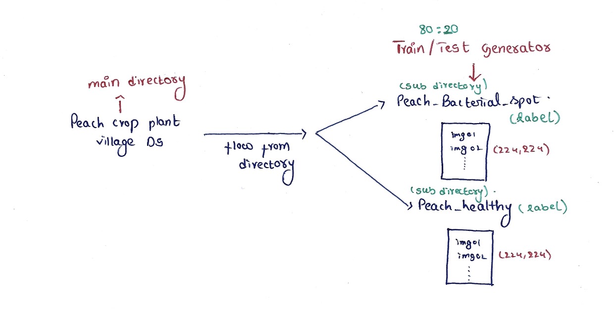
The images loaded will be of size (224, 224) and rescaled between '0 and 1' and batched into 64 and 32 for train and test respectively. Further preprocessing is not required😁.

crop_directory = 'Peach Crop plant Village DS'

train_generator = datagen.flow_from_directory(
    crop_directory,
    target_size = (224,224),
    batch_size = 64,
    class_mode = 'binary',
    shuffle = True,
    subset = 'training'
)

test_generator = datagen.flow_from_directory(
    crop_directory,
    target_size = (224,224),
    batch_size = 32,
    class_mode = 'binary',
    shuffle = True,
    subset = 'validation'
)

Output :

Found 2126 images belonging to 2 classes.

Found 531 images belonging to 2 classes.

Defining Architecture

As we discussed above, CNN architecture is a good choice for tasks like image classification.

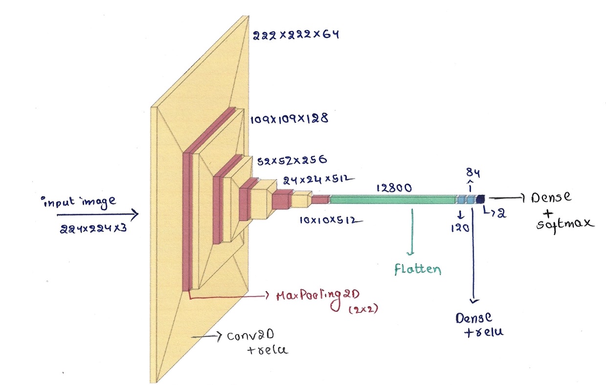
Activation Functions Used:

ReLU is used as the activation function in Convolutional layers and the hidden layers of fully connected layers. As the ReLU activation function overcomes the vanishing gradient problem, allowing models to learn faster and perform better. It is almost the default activation when developing multilayer Perceptron and convolutional neural networks. Learn more about why ReLU is preferred over Other activation functions

Softmax is used as the activation function in the output layer as it gives probabilistic output. ( For this model as it is binary classification, you can also use the sigmoid activation function in the output layer☺️ but don't forget to change the number of neurons to 1🙃 for sigmoid)

For more justification please refer to this paper: On Approximation Capabilities of ReLU Activation and Softmax Output Layer in Neural Networks

model = Sequential()

model.add(Conv2D(64,(3,3),activation='relu',input_shape=(224,224,3)))
model.add(MaxPooling2D(2,2))

model.add(Conv2D(128,(3,3),activation='relu'))
model.add(MaxPooling2D(2,2))

model.add(Conv2D(256,(3,3),activation='relu'))
model.add(MaxPooling2D(2,2))

for i in range(2):
    model.add(Conv2D(512,(3,3),activation='relu'))
    model.add(MaxPooling2D(2,2))

model.add(Flatten())
model.add(Dense(120,activation='relu'))
model.add(Dense(84,activation='relu'))
model.add(Dense(2,activation='softmax'))

COMPILE MODEL

Compiling a model is the process of configuring it for training. It involves specifying the optimizer, loss function, and metrics that will be used.

Optimizer: The optimizer is an algorithm that updates the weights of the model during training : Adam The Adam optimizer is a popular choice for training Keras models.

Loss function: The loss function is a measure of how well the model is performing on the training data : sparse_categorical_crossentropy. This loss function is suitable for multi-class classification problems.

Metrics: The metrics are used to evaluate the performance of the model on the training and validation data.['accuracy']. The accuracy metric measures the percentage of predictions that are correct.

model.compile(
    optimizer = 'adam',
    loss = 'sparse_categorical_crossentropy',
    metrics = ['accuracy']
)

TRAIN THE MODEL

Callbacks

Suppose, we are training our model for some 50 epochs... and we are willing to attain the accuracy of some 0.9800...😉 If our model can achieve the required accuracy within 15 - 20 epochs, It is a waste of resources and time to run the other 30 epochs. So we have to stop training after we achieve the required accuracy.

We can achieve this by using Callbacks. It checks the accuracy at the end of each epoch and if the required accuracy is reached, the training will be stopped.

class myCallback(tf.keras.callbacks.Callback):
    def on_epoch_end(self,epoch,logs={}):
        if(logs.get('accuracy')>=0.9800):
            print('\nReached accuracy of 0.9800. So we  stop the Training.')
            self.model.stop_training = True


stop_at = myCallback()

FITTING

Now we train the model by fitting the features of the images to the label and iteratively adjust weights and bias to find the perfect fit to determine a new image to the available label categories.

fit(): Trains the model on the given data.
train_generator: A generator that yields batches of training data.
steps_per_epoch: The number of batches of training data to use per epoch.
epochs: The number of times to train the model on the entire training dataset.
validation_data: A generator that yields batches of validation data. ( Which is the data that was not used to train the model and used to evaluate model performance)
validation_steps: The number of batches of validation data to use per epoch.
callbacks: A list of callback functions that are invoked during training.
stop_at (defined by us): A callback function that stops training early if the desired accuracy is reached.
history: A dictionary containing the training history, such as the training and validation loss and accuracy.

history = model.fit(
    train_generator,
    steps_per_epoch = len(train_generator),
    epochs = 50,
    validation_data = test_generator,
    validation_steps = len(test_generator),
    callbacks = [stop_at]
)

Epoch 1/50

34/34 [==============================] - 202s 6s/step - loss: 0.3403 - accuracy: 0.8829 - val_loss: 0.1435 - val_accuracy: 0.9322

Epoch 2/50

34/34 [==============================] - 212s 6s/step - loss: 0.1658 - accuracy: 0.9393 - val_loss: 0.0809 - val_accuracy: 0.9755

...............................................................

Epoch 15/50

34/34 [==============================] - 289s 9s/step - loss: 0.0553 - accuracy: 0.9765 - val_loss: 0.0554 - val_accuracy: 0.9718

Epoch 16/50 34/34 [==============================] - 281s 8s/step - loss: 0.0513 - accuracy: 0.9774 - val_loss: 0.0371 - val_accuracy: 0.9831

Epoch 17/50 34/34 [==============================] - 281s 8s/step - loss: 0.0413 - accuracy: 0.9859 - val_loss: 0.0390 - val_accuracy: 0.9849

MODEL PERFORMANCE

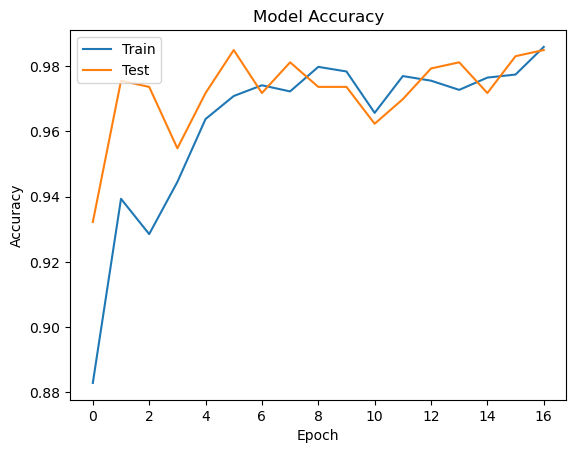
To evaluate model performance, We plot the model accuracy and loss graphs which show the model accuracy and loss on train and test data.

plt.plot(history.history['accuracy'])
plt.plot(history.history['val_accuracy'])
plt.title('Model Accuracy')
plt.xlabel('Epoch')
plt.ylabel('Accuracy')
plt.legend(['Train','Test'],loc="upper left")
plt.show()

plt.plot(history.history['loss'])
plt.plot(history.history['val_loss'])
plt.title('Model Loss')
plt.xlabel('Epoch')
plt.ylabel('Loss')
plt.legend(['Train','Test'],loc="upper left")
plt.show()

MODEL ACCURACY

MODEL LOSS

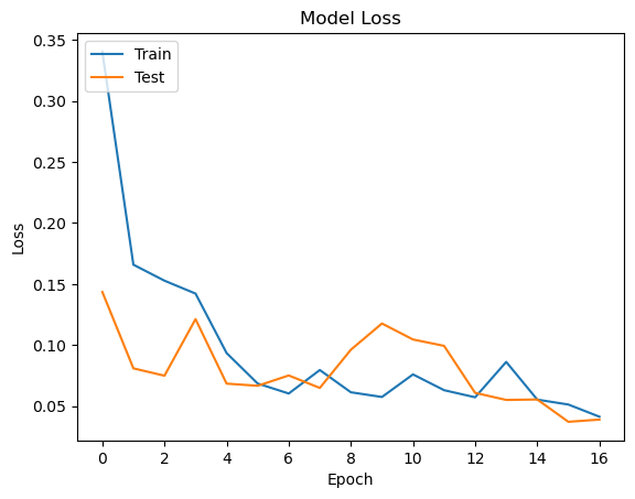
INFERENCE:

Overall, the accuracy of our model is very impressive. This suggests that we have trained a robust and reliable model that can be used to make accurate predictions in real-world settings🥳

The loss graph of our model shows that the model is learning well and converging to a low loss value. The loss value on the training set is lower than the loss value on the test set, which is a good sign. It indicates that the model is not overfitting to the training data and can generalize well to new data.

The loss and accuracy graphs of your model suggest that you have trained a successful model. The model is learning well, generalizing well to new data, and making accurate predictions.

So, our model can be useful to detect the infected peach crop plants by taking the image of the leaf as input. Which can be very helpful to the farmers to prevent the spread of the disease to the neighbouring plants of the crop.

💡

You can get the notebook file here

Thank you.

Save Your Peach Crops from Infection with This Simple TensorFlow CNN Model

Table of contents