QUICK sort

Before delving into the intricacies of quick sort, I'd like to address your queries. Indeed, quick sort operates in O(n log n) time complexity and, in practical scenarios, it often outperforms both merge sort and heap sort in terms of speed.

SPOILER: For sorting 1 million elements, Bubble Sort requires approximately 3 hours, whereas Quick Sort needs only about 0.2 seconds.

Now, to understand quick sort effectively, we need to focus on three crucial elements:

1. Pivot Selection

2. Division into Two Parts

3. Recursion

Let's explore quick sort by examining these three aspects.

Understanding the Function and Determination of the Pivot

In quick sort, the pivot can be the first, last, middle, or a randomly chosen element. In small datasets, the choice of pivot doesn't significantly impact performance. However, for larger datasets, a random pivot is often a superior choice. For our explanation, we'll select the first element as the pivot to understand its role and functionality.

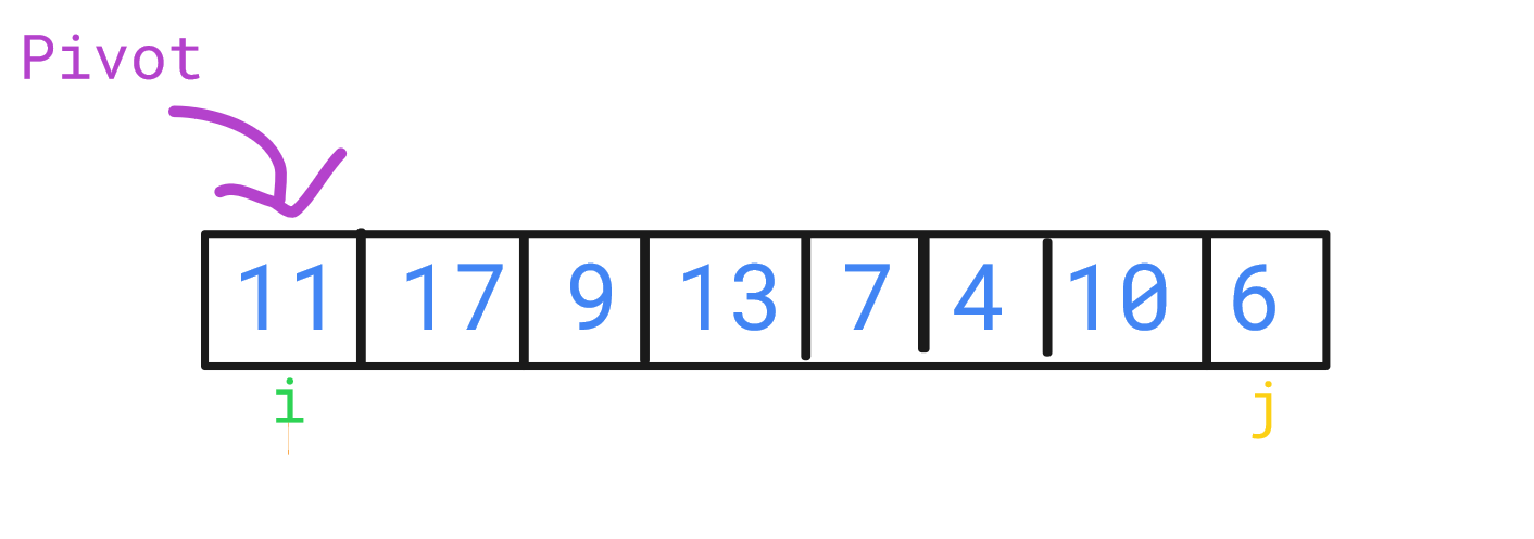
Consider the following array:

11, 17, 9, 13, 16, 7, 4, 10, 6

Here, the pivot is the first element: 11.

We use two pointers, i and j, to find elements greater and smaller than the pivot, respectively. These elements are then swapped. But when do i and j stop and swap their elements? The answer lies in their comparison with the pivot. For instance, in our array, 17 (greater than 11) and 6 (less than 11) are candidates for swapping. After this swap, the array looks like:

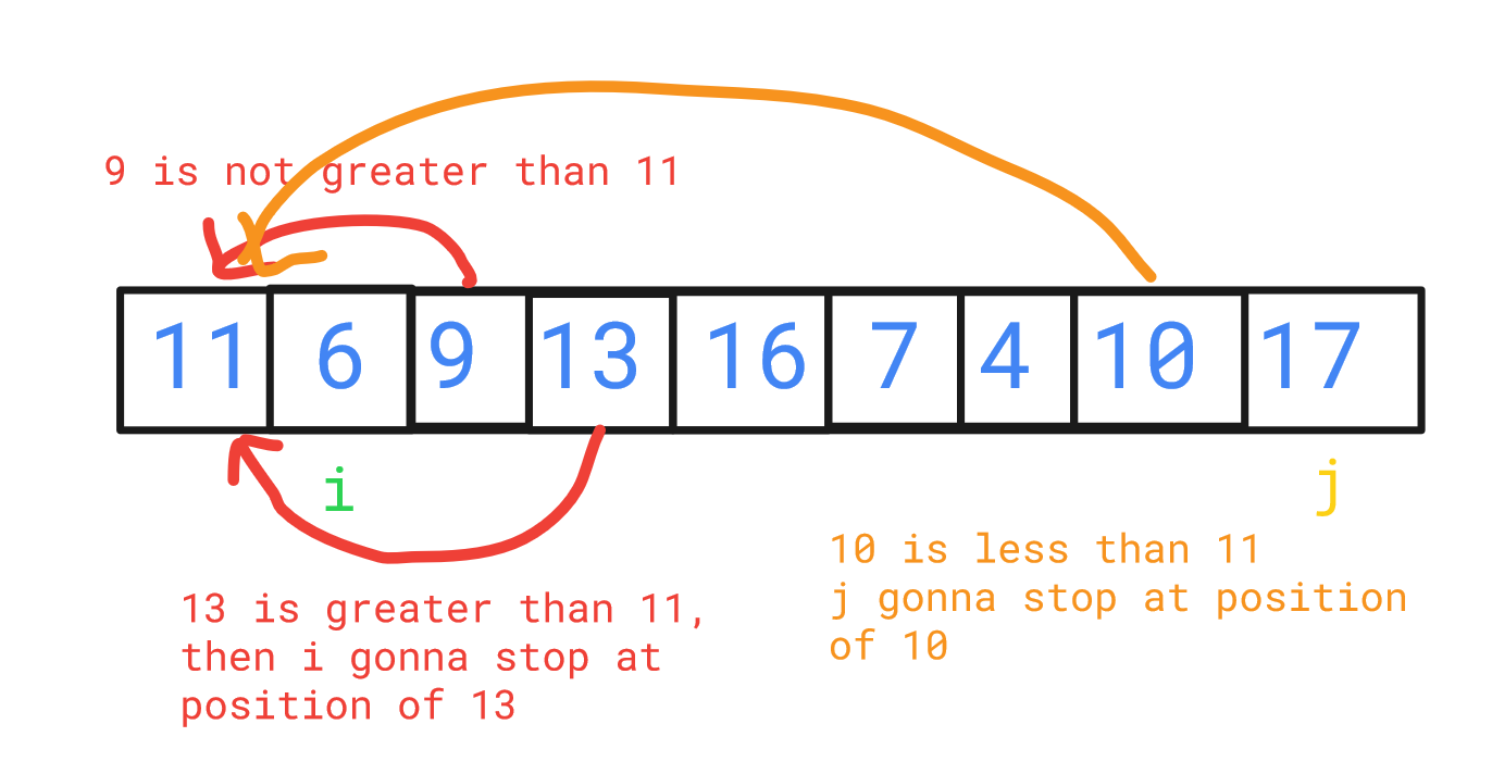
11, 6, 9, 13, 16, 7, 4, 10, 17

This process continues. We check from the left: 9 is not greater than 11, but 13 is, so i stops here. From the right: 10 is less than 11, so j stops there. We swap these elements:

11, 6, 9, 10, 16, 7, 4, 13, 17

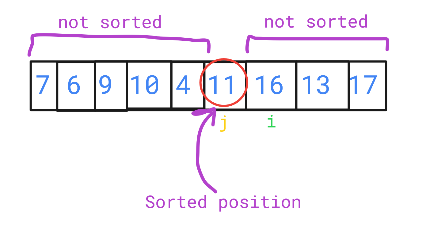
Following this pattern, when i and j cross, it indicates the final position for the pivot. In our example, 11 swaps with 4, resulting in:

7, 6, 9, 10, 4, 11, 16, 13, 17

Although the entire array isn't sorted yet, 11 is in its correct position. By recursively applying this process to the left and right sides of the pivot, the entire array can be sorted. This method is known as partitioning.

def partition(array, low, high):
    pivot = array[high] # Rightmost element as pivot
    i = low - 1
    for j in range(low, high):
        if array[j] <= pivot:
            i += 1
            array[i], array[j] = array[j], array[i]
    array[i + 1], array[high] = array[high], array[i + 1]
    return i + 1

Use a recursive function, say quickSort, to initiate the sorting process. The partition function divides the array, and the quickSort function is recursively called for the left and right halves of the partition.

def quicksort(array, low, high):
    if low < high:
        pi = partition(array, low, high)
        quicksort(array, low, pi - 1)
        quicksort(array, pi + 1, high)

Complexity Analysis

• Best Case: Ω(N log N)

• Average Case: θ(N log N)

• Worst Case: O(N²)

A notable drawback of quick sort is its NOT STABLE; it does not maintain the relative order of equal elements.

Let's compare Quick sort with Bubble sort in very simple way:

To calculate the actual time in minutes, we need to know the number of operations the processor can handle per second. Let's assume a modern processor can perform approximately 10^8 operations per second. Using this, we can estimate the time taken by each algorithm.

The estimated time for sorting a dataset of 1 million elements using Bubble Sort is approximately 166.67 minutes, while using Quick Sort, it's about 0.0033 minutes (approximately 0.2 seconds).