Optimizing PostgreSQL Performance: BRIN vs B-tree Indexing Case Study

Introduction

PostgreSQL, known for its extensibility and robustness, offers a variety of indexing options to optimize query performance. Among these, Block Range INdexes (BRIN) provide a unique approach to indexing large tables with ranges of values. In this blog, we'll talk about BRIN indexes, look at a real-life example to see how they perform compared to regular B-tree indexes, and discuss when it's not a good idea to use them.

Understanding BRIN Indexes

Block Range INdexes are designed to efficiently index large tables with sorted ranges of data, such as chronological or numerical data. Unlike B-tree indexes that store individual values, BRIN indexes divide the table into fixed-size blocks and store summary information for each block. This makes BRIN indexes particularly well-suited for scenarios where data exhibits natural ordering, such as timestamp-based or sequential data.

Data in PostgreSQL tables are arranged on disk in equal-sized "pages" of 8kb each. So a table will physically reside on disk as a collection of pages. Within each page, rows are packed in from the front, with gaps appearing as data is deleted/updated and usually some spare space at the end for future updates.

A table with narrow rows (few columns, small values) will fit a lot of rows into a page. A table with wide rows (more columns, long strings) will fit only a few.

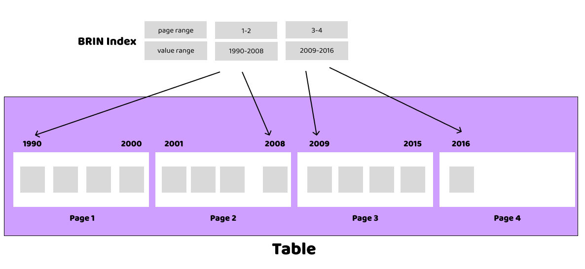
Because each page holds multiple rows, we can state that a given column on that page has a minimum and maximum value on that page. When searching for a particular value, the whole page can be skipped, if the value is not within the min/max of the page. This is the core magic of BRIN.

So, for BRIN to be effective, you need a table where the physical layout and the ordering of the column of interest are strongly correlated. In the situation of perfect correlation (which we test below), each page will contain a unique set of values.

The BRIN index is a small table that associates a range of values with a range of pages in the table order. Building the index just requires a single scan of the table, so compared to building a structure like a BTree, it is very fast.

Because the BRIN has one entry for each range of pages, it's also very small. The number of pages in a range is configurable, but the default is 128. Tuning this number can make a big difference in query performance.

Comparing BRIN and B-tree Index Performance

Let's consider a real-world case to showcase the performance difference between BRIN and B-tree indexes. Imagine a scenario where you have a large table storing time-series data, and you need to retrieve records within a specific date range.

Setting up the Scenario

Let's create two tables one with a B-tree index and one with a BRIN index.

Tables: sensor_data_1 & sensor_data_2
Columns: timestamp (time of data capture), sensor_id, value

-- create table sensor_data_1
CREATE TABLE sensor_data_1(
  sensor_id INT PRIMARY KEY, 
  value TEXT, 
  timestamp TIMESTAMP
);

-- create table sensor_data_2
CREATE TABLE sensor_data_2(
  sensor_id INT PRIMARY KEY, 
  value TEXT, 
  timestamp TIMESTAMP
);

Creating B-tree Index

CREATE INDEX btree_timestamp_idx ON sensor_data_1(timestamp);

Creating BRIN Index

CREATE INDEX brin_timestamp_idx ON sensor_data_2 USING brin(timestamp);

Populate data

Now let us insert some random data that is incremental. The below query generates 1 million rows sensor_id ranging from 1 to 1000000, a sample text value, and a timestamp that increases by a second with each row. You can adjust the number in the generate_series function to generate more or fewer rows as needed.

-- insert data to sensor_data_1
INSERT INTO sensor_data_1(sensor_id, value, timestamp)
SELECT
  gs.n AS sensor_id,
  'Sample Value ' || gs.n AS value,
  NOW() + (gs.n || ' seconds')::INTERVAL AS timestamp
FROM generate_series(1, 1000000) AS gs(n);

-- insert data to sensor_data_2
INSERT INTO sensor_data_2(sensor_id, value, timestamp)
SELECT
  gs.n AS sensor_id,
  'Sample Value ' || gs.n AS value,
  NOW() + (gs.n || ' seconds')::INTERVAL AS timestamp
FROM generate_series(1, 1000000) AS gs(n);

Performance Test Query

EXPLAIN ANALYZE SELECT * FROM sensor_data_1 WHERE timestamp BETWEEN '2024-01-01' AND '2024-01-05';

"Index Scan using btree_timestamp_idx on sensor_data_1  (cost=0.42..19999.10 rows=521584 width=31) (actual time=0.022..109.712 rows=518400 loops=1)"
"  Index Cond: ((""timestamp"" >= '2024-01-01 00:00:00'::timestamp without time zone) AND (""timestamp"" <= '2024-01-07 00:00:00'::timestamp without time zone))"
"Planning Time: 0.066 ms"
"Execution Time: 135.485 ms"

EXPLAIN ANALYZE SELECT * FROM sensor_data_2 WHERE timestamp BETWEEN '2024-01-01' AND '2024-01-05';

"Bitmap Heap Scan on sensor_data_2  (cost=98.99..12883.02 rows=345257 width=31) (actual time=0.350..70.053 rows=345600 loops=1)"
"  Recheck Cond: ((""timestamp"" >= '2024-01-01 00:00:00'::timestamp without time zone) AND (""timestamp"" <= '2024-01-05 00:00:00'::timestamp without time zone))"
"  Rows Removed by Index Recheck: 19968"
"  Heap Blocks: lossy=2688"
"  ->  Bitmap Index Scan on brin_timestamp_idx  (cost=0.00..12.67 rows=362069 width=0) (actual time=0.051..0.051 rows=26880 loops=1)"
"        Index Cond: ((""timestamp"" >= '2024-01-01 00:00:00'::timestamp without time zone) AND (""timestamp"" <= '2024-01-05 00:00:00'::timestamp without time zone))"
"Planning Time: 0.063 ms"
"Execution Time: 86.876 ms"

As we can see in scenarios where the data is naturally ordered, BRIN indexes can demonstrate significant performance benefits due to their block-based structure. In this case, the size of the tables was 1 million rows. Lager the table larger will be the benefit.

Index size comparison

-- size of the table
SELECT pg_size_pretty(pg_relation_size('sensor_data_2'))

"57 MB"

-- size of the b-tree index
SELECT pg_size_pretty(pg_relation_size('btree_timestamp_idx'));

"21 MB"

-- size of the brin index
SELECT pg_size_pretty(pg_relation_size('brin_timestamp_idx'));

"24 kB"

The BTree indexes end up very close to the table size. The BRIN indexes are 1000 times smaller.

Scenario: Highly Unordered Data

Let's explore a case where using BRIN indexes in the wrong context can lead to suboptimal performance. Consider a table with randomly distributed data, such as a user profile table with no clear ordering. In this case, using a BRIN index might result in poor performance compared to a B-tree index.

Let's create two tables one with a B-tree index and one with a BRIN index.

Tables: user_profile_1 & user_profile_2
Columns: username, age, city

-- create table user_profile_1
CREATE TABLE user_profile_1(
  username TEXT, 
  age TEXT, 
  city TEXT
);

-- create table user_profile_2
CREATE TABLE user_profile_2(
  username TEXT, 
  age TEXT, 
  city TEXT
);

Creating indexes:

-- create b-tree index on user_profile_1
CREATE INDEX btree_username_idx ON user_profile_1(username);

-- create brin index on user_profile_2
CREATE INDEX brin_username_idx ON user_profile_2 USING brin(username);

Populating data:

-- insert data to user_profile_1
INSERT INTO user_profile_1(username, age, city)
SELECT
  md5(random()::text || clock_timestamp()::text)::uuid::text,  -- Generate random username
  floor(random() * 100)::text,                                  -- Generate random age (0 to 99)
  CASE 
    WHEN random() < 0.33 THEN 'New York'
    WHEN random() < 0.66 THEN 'Los Angeles'
    ELSE 'Chicago'
  END                                                           -- Randomly select city
FROM generate_series(1, 1000000);

-- insert data to user_profile_2
INSERT INTO user_profile_2(username, age, city)
SELECT
  md5(random()::text || clock_timestamp()::text)::uuid::text,  -- Generate random username
  floor(random() * 100)::text,                                  -- Generate random age (0 to 99)
  CASE 
    WHEN random() < 0.33 THEN 'New York'
    WHEN random() < 0.66 THEN 'Los Angeles'
    ELSE 'Chicago'
  END                                                           -- Randomly select city
FROM generate_series(1, 1000000);

Check performance:

EXPLAIN ANALYZE SELECT * FROM user_profile_1 WHERE username = '2df777d2-c8a9-53da-4174-da56a42c5c0a';

"Index Scan using btree_username_idx on user_profile_1  (cost=0.42..8.44 rows=1 width=49) (actual time=1.972..1.974 rows=1 loops=1)"
"  Index Cond: (username = '2df777d2-c8a9-53da-4174-da56a42c5c0a'::text)"
"Planning Time: 0.059 ms"
"Execution Time: 2.559 ms"

EXPLAIN ANALYZE SELECT * FROM user_profile_2 WHERE username = '2df777d2-c8a9-53da-4174-da56a42c5c0a';

"Gather  (cost=1000.00..16285.43 rows=1 width=49) (actual time=94.035..99.614 rows=0 loops=1)"
"  Workers Planned: 2"
"  Workers Launched: 2"
"  ->  Parallel Seq Scan on user_profile_2  (cost=0.00..15285.33 rows=1 width=49) (actual time=41.383..41.384 rows=0 loops=3)"
"        Filter: (username = '2df777d2-c8a9-53da-4174-da56a42c5c0a'::text)"
"        Rows Removed by Filter: 333333"
"Planning Time: 22.366 ms"
"Execution Time: 99.638 ms"

In scenarios where the data lacks a clear range-based order, BRIN indexes might lead to increased I/O operations and decreased query performance compared to B-tree indexes.

Tuning Parameters

The pages_per_range parameter determines how many consecutive pages of the table should be covered by a single BRIN range(default is 128). Adjusting this parameter allows you to balance the trade-off between index size and query performance.

A smaller value pages_per_range results in a more granular index, potentially allowing for more precise range filtering.
A larger value reduces the number of summary entries in the index, leading to a more compact index but potentially sacrificing precision in range queries.

Creating BRIN Index with Tuned pages_per_range

CREATE INDEX brin_timestamp_tuned_idx ON sensor_data USING brin(timestamp) WITH (pages_per_range = 100);

Tuning the pages_per_range parameter allows you to tailor the BRIN index to the specific characteristics of your dataset. It's an ongoing process that involves monitoring and experimenting to strike the right balance between precision and index size. By fine-tuning this parameter, you can further optimize the performance of BRIN indexes and enhance the overall efficiency of your PostgreSQL database.

Conclusion

Understanding the strengths and limitations of indexing techniques is crucial for optimizing database performance. BRIN indexes offer a powerful solution for certain use cases, particularly those involving range-based data. However, as demonstrated in our case study, using BRIN indexes inappropriately can lead to diminished performance. It's essential to carefully evaluate the nature of your data and choose the indexing strategy that aligns with its characteristics to harness the full potential of PostgreSQL's indexing capabilities.

Boosting PostgreSQL Performance with BRIN Indexes