How to Make an Automatic Speech Recognition System with Wav2Vec 2.0 on E2E’s Cloud GPU Server

Introduction

Creating an Automatic Speech Recognition (ASR) system using Wav2Vec 2.0 on E2E’s Cloud GPU server is a compelling endeavor that brings together cutting-edge technology and robust infrastructure. Leveraging the power of Wav2Vec 2.0, a state-of-the-art framework for self-supervised learning of speech representations, and harnessing the capabilities of E2E’s Cloud GPU server, this guide will walk you through the process of developing an efficient ASR system. From setting up the necessary components to fine-tuning your model on the cloud, this article will provide a comprehensive overview, enabling you to harness the potential of ASR for diverse applications.

Let’s embark on a journey to build a high-performance Automatic Speech Recognition System on E2E’s Cloud GPU server.

Automatic Speech Recognition System

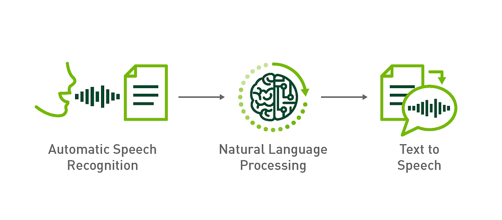
Automatic Speech Recognition (ASR) is a technology that empowers computers to interpret and transcribe spoken language into written text. This innovative field, falling under the umbrella of computational linguistics, plays a pivotal role in applications ranging from voice-to-text dictation software to virtual assistants, call center systems, transcription services, and accessibility tools. Additionally, ASR systems can be employed for speech synthesis, generating spoken language from text or other inputs.

Types of ASR Systems

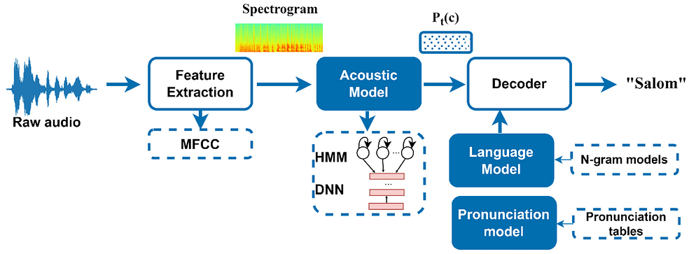
1. Rule-Based ASR: Rule-based Automatic Speech Recognition (ASR) employs predefined rules and patterns to match acoustic features with linguistic units, prioritizing simplicity and speed. While effective in well-defined language and low-noise scenarios, it has limitations such as a restricted vocabulary and struggles with noisy or ambiguous speech. Consequently, rule-based ASR excels in specific contexts but may not be ideal for applications demanding flexibility in vocabulary or robust performance in challenging acoustic conditions.

2. Statistical ASR: Statistical Automatic Speech Recognition (ASR) utilizes statistical models to map acoustic features to linguistic units, demonstrating adaptability with variable vocabulary sizes and noise resilience. While versatile, it requires substantial training data and computational resources for accurate models. The statistical approach enables the system to extract intricate patterns from diverse datasets, enhancing its flexibility in transcribing speech. This makes statistical ASR well-suited for applications dealing with varying vocabulary sizes and common challenges like ambient noise.

3. Neural Network-Based ASR: Neural network-based Automatic Speech Recognition (ASR) utilizes deep learning to achieve high accuracy and robust performance in transcribing speech. By discerning intricate patterns in speech signals, it excels in recognizing nuances. However, this heightened performance requires substantial training data and computational resources. The training process involves exposing the network to large, diverse datasets, demanding significant computational power. Despite its resource-intensive nature, neural network-based ASR is a formidable choice for applications prioritizing precision and adaptability in handling diverse linguistic patterns.

Examples of Neural Network-Based ASR Models

1. Transformer-Based ASR: Transformer-based Automatic Speech Recognition (ASR) employs attention mechanisms to capture long-range dependencies between acoustic features and linguistic units. This approach has demonstrated exceptional performance, achieving state-of-the-art results on benchmark datasets like LibriSpeech and Common Voice. The use of attention mechanisms allows the model to effectively analyze and incorporate information from distant parts of the input, enhancing its ability to transcribe spoken language with high accuracy and efficiency.

2. CNN-Based ASR: CNN-based Automatic Speech Recognition (ASR) utilizes convolutional filters to extract local features from acoustic signals and can be seamlessly combined with RNNs or transformers. This approach excels in handling variable-length sequences and effectively addresses long-term dependencies in speech data. By leveraging convolutional filters, the model efficiently captures local patterns, while its compatibility with other architectures enhances its adaptability to diverse speech recognition challenges.

3. Hybrid Neural Network-Based ASR: Hybrid Automatic Speech Recognition (ASR) combines various neural network architectures to capitalize on their individual strengths and mitigate limitations. An illustrative example involves integrating Recurrent Neural Networks (RNNs) to handle short-term dependencies and transformers to address long-term dependencies. This hybrid approach allows the system to benefit from the complementary features of different architectures, enhancing its overall performance and adaptability in recognizing and transcribing spoken language.

Wav2Vec2.0: Self-Supervised Speech Learning

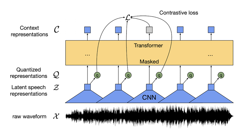
Wav2Vec 2.0 represents a cutting-edge framework for self-supervised learning of speech representations, offering a revolutionary approach to extracting meaningful features from speech audio without relying on human annotations or labeled data. The framework is underpinned by the innovative concept of contrastive learning, a technique that enables the model to distinguish between similar and dissimilar inputs. This is achieved by maximizing the similarity between positive pairs (e.g., different segments of the same speaker) while simultaneously minimizing the similarity between negative pairs (e.g., representations from different speakers).

Components

1. Speech Encoder: The speech encoder is a neural network designed to take raw audio as input and produce a latent representation — a compact, high-dimensional vector capturing the essential characteristics of the speech signal.

2. Contrastive Loss Function: The contrastive loss function evaluates the fidelity of this representation by comparing it to ground truth transcriptions, considering other latent representations from different speakers or segments.

Components of Wav2Vec 2.0

Architecture

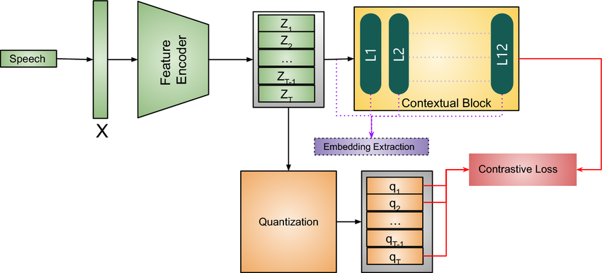
The architecture of Wav2Vec 2.0 is designed to facilitate self-supervised learning of speech representations. Here are the key components of its architecture:

1. Multi-Layer Convolutional Feature Encoder (f: X → Z): The model begins with a multi-layer convolutional feature encoder. This encoder, denoted as f: X → Z, takes raw audio input X and produces latent speech representations z_1,…,z_T time-steps. These representations capture essential characteristics of the speech signal.

2. Transformer (g: Z → C) for Contextualized Representations: The latent speech representations z_1,…,z_T are then fed into a Transformer network, denoted as g: Z → C, to build contextualized representations c_1,…,c_T. The Transformer architecture is known for its effectiveness in capturing dependencies over entire sequences.

3. Quantization Module (Z → Q): The output of the feature encoder is discretized using a quantization module Z → Q. This module involves selecting quantized representations from multiple codebooks and concatenating them. The process is facilitated by a Gumbel softmax, which allows for the differentiable selection of discrete codebook entries.

Architecture of Wav2Vec 2.0

4. Gumbel Softmax for Discrete Codebook Entries: The Gumbel softmax is employed for choosing discrete codebook entries in a fully differentiable manner. The straight-through estimator and G hard Gumbel softmax operations are used during training. This mechanism enables the model to choose discrete codebook entries while maintaining differentiability for effective training.

5. Contextualized Representations with Transformers: The output of the feature encoder is further processed by a context network, following the Transformer architecture. This network incorporates relative positional information using a convolutional layer and adds the output to the inputs, followed by a GELU activation function and layer normalization.

The Need of a Cloud GPU

Automatic Speech Recognition (ASR) is a technology enabling computers to convert spoken language into written text, falling within the domain of computational linguistics. ASR finds diverse applications, including voice-to-text dictation, virtual assistants, call centers, transcription services, and accessibility tools. ASR faces challenges due to the complexity and variability of speech signals, necessitating advanced techniques to extract meaningful features and map them to linguistic units.

Deep learning, a popular approach in ASR, involves neural networks that learn hierarchical representations from raw or preprocessed audio data, capturing both low-level acoustic features and high-level semantic features. However, deep learning models demand significant computational resources. GPU-accelerated ASR addresses this by utilizing graphics processing units (GPUs) to expedite the training and inference processes. This acceleration enhances recognition accuracy, even on embedded and mobile systems, and facilitates rapid transcription of pre-recorded speech or multimedia content.

A dedicated cloud GPU for ASR brings several advantages over general-purpose CPUs or other hardware devices:

1. Efficient Handling of Large-Scale Datasets: GPUs efficiently handle large-scale datasets with scalability.

2. Support for Multiple Models: GPUs can support multiple models with varying architectures and parameters.

3. Reduced Latency and Bandwidth Consumption: Distributing workload across multiple GPUs reduces latency and bandwidth consumption.

1. Real-time or Near-Real-time Applications: Cloud GPUs enable real-time or near-real-time applications that demand fast response times.

E2E Networks: Advanced Cloud GPU

E2E Networks stands as a prominent hyperscaler from India, specializing in state-of-the-art Cloud GPU infrastructure. Their offerings include cutting-edge Cloud GPUs such as A100/V100/H100 and the AI Supercomputer HGX 8xH100 GPUs, providing accelerated cloud computing solutions. E2E Networks offers a diverse range of advanced cloud GPUs at highly competitive rates. For detailed information on the products available from E2E Networks, visit their website. When choosing the optimal GPU for implementing the Automatic Speech Recognition System, the decision should be based on your specific requirements and budget. In my case, I utilized a GPU dedicated compute with V100–8–120 GB with Cuda 11 for efficient performance.

To know in detail how to use E2E cloud GPUs, visit my previous article.

First, log in remotely with SSH on your local system. Now, let’s start implementing the code.

Implementing ASR with Wav2Vec 2.0

First, install all the libraries which are required in our code implementation.

%pip install -q torch numpy transformers datasets evaluate

Import all the packages that we are going to need in our implementation.

from datasets import load_dataset, Audio
from transformers import AutoProcessor
import torch
from dataclasses import dataclass, field
from typing import Any, Dict, List, Optional, Union
import evaluate
import numpy as np
from transformers import AutoModelForCTC, TrainingArguments, Trainer
from transformers import pipeline

I have taken a multilingual ASR dataset from Hugging Face. You can find the dataset here.

Load the dataset.

data= load_dataset("google/fleurs", name="en_us", split="train[:100]")

Let’s split the dataset, so that we can put the test set for evaluation.

data= data.train_test_split(test_size=0.2)

Next, we’ll load a Wav2Vec2 processor to handle the audio signal.

processor = AutoProcessor.from_pretrained("facebook/wav2vec2-base")

Then we’ll resample the dataset to 16000 HZ to use the pretrained Wav2Vec2 model.

data= data.cast_column("audio", Audio(sampling_rate=16000))

The dataset’s transcription is in lowercase. The Wav2Vec2 tokenizer is only trained on uppercase characters so we’ll need to make sure the text matches the tokenizer’s vocabulary.

def uppercase(example):
 return {"transcription": example["transcription"].upper()}

data= data.map(uppercase)

Now, generate a preprocessing function that:

1. Invokes the audio column to load and resample the audio file.

2. Retrieves the input_values from the audio file and tokenizes the transcription column using the processor.

def prepare_dataset(batch):
 audio = batch["audio"]
 batch = processor(audio["array"], sampling_rate=audio["sampling_rate"], text=batch["transcription"])
 batch["input_length"] = len(batch["input_values"][0])
 return batch

To employ the preprocessing function across the complete dataset, utilize the Datasets map function. Enhance the mapping efficiency by adjusting the number of processes through the num_proc parameter.

encoded_data = data.map(prepare_dataset, num_proc=4)

Transformers currently lack a dedicated data collator for ASR, necessitating the adaptation of DataCollatorWithPadding to construct a batch of examples. This adapted collator dynamically pads text and labels to the length of the longest element within the batch, ensuring uniform length, as opposed to the entire dataset. Although padding in the tokenizer function is achievable by setting padding=True, dynamic padding proves to be more efficient.

Distinct from other data collators, this specific collator must employ a distinct padding method for input_values and labels:

# Define a data collator for CTC (Connectionist Temporal Classification) with padding
@dataclass
class DataCollatorCTCWithPadding:
 # AutoProcessor is expected to be a processor for audio data, e.g., from Hugging Face transformers library
 processor: AutoProcessor
 # padding parameter can be a boolean or a string, defaults to "longest"
 padding: Union[bool, str] = "longest"
 # __call__ method is used to make an instance of the class callable
 def __call__(self, features: List[Dict[str, Union[List[int], torch.Tensor]]]) -> Dict[str, torch.Tensor]:
 # Split inputs and labels since they have to be of different lengths and need different padding methods
 input_features = [{"input_values": feature["input_values"][0]} for feature in features]
 label_features = [{"input_ids": feature["labels"]} for feature in features]
 # Pad input features using the processor
 batch = self.processor.pad(input_features, padding=self.padding, return_tensors="pt")
 # Pad label features using the processor
 labels_batch = self.processor.pad(labels=label_features, padding=self.padding, return_tensors="pt")
 # Replace padding with -100 to ignore loss correctly
 labels = labels_batch["input_ids"].masked_fill(labels_batch.attention_mask.ne(1), -100)
 # Add labels to the batch
 batch["labels"] = labels
 return batch

Now instantiate your DataCollatorForCTCWithPadding.

data_collator = DataCollatorCTCWithPadding(processor=processor, padding="longest")

Incorporating a metric during training is frequently beneficial for assessing your model’s performance. You can effortlessly load an evaluation method using the Evaluate library. For this particular task, load the Word Error Rate (WER) metric.

wer = evaluate.load("wer")

Then create a function that passes your predictions and labels to compute to calculate the WER.

# Define a function to compute metrics (Word Error Rate in this case) for model evaluation
def compute_metrics(pred):
 # Extract predicted logits from the predictions
 pred_logits = pred.predictions
 # Convert logits to predicted token IDs by taking the argmax along the last axis
 pred_ids = np.argmax(pred_logits, axis=-1)
 # Replace padding in label IDs with the tokenizer's pad token ID
 pred.label_ids[pred.label_ids == -100] = processor.tokenizer.pad_token_id
 # Decode predicted token IDs into strings
 pred_str = processor.batch_decode(pred_ids)
 # Decode label token IDs into strings without grouping tokens
 label_str = processor.batch_decode(pred.label_ids, group_tokens=False)
 # Compute Word Error Rate (WER) using the wer.compute function
 wer = wer.compute(predictions=pred_str, references=label_str)
 # Return the computed metric (WER) as a dictionary
 return {"wer": wer}

Load Wav2Vec2 using AutoModelForCTC. Specify the reduction to apply with the ctc_loss_reduction parameter. It is typically preferable to use the average instead of the default summation.

model = AutoModelForCTC.from_pretrained(
 "facebook/wav2vec2-base",
 ctc_loss_reduction="mean",
 pad_token_id=processor.tokenizer.pad_token_id,
)

To store your fine-tuned model, make a directory.

%mkdir my_model

At this stage, the final three steps in the process involve setting up your training hyperparameters in TrainingArguments, with the essential parameter being output_dir, specifying the model’s saving location. If you intend to share your model on the Hugging Face Hub, simply set push_to_hub=True, ensuring that you are signed in to Hugging Face for the upload.

# Enable gradient checkpoints for memory efficiency during training
model.gradient_checkpoints_enable()
# Define training arguments for the Trainer class
training_args = TrainingArguments(
 output_dir="my_model", # Directory to save the trained model
 per_device_train_batch_size=8, # Batch size per GPU device during training
 gradient_accumulation_steps=2, # Number of updates to accumulate before performing a backward/update pass
 learning_rate=1e-5, # Learning rate for the optimizer
 warmup_steps=500, # Number of steps for warm-up in the learning rate scheduler
 max_steps=2000, # Maximum number of training steps
 fp16=True, # Enable mixed-precision training using 16-bit floats
 group_by_length=True, # Group batches by input sequence length for efficiency
 evaluation_strategy="steps", # Evaluate the model every specified number of training steps
 per_device_eval_batch_size=8, # Batch size per GPU device during evaluation
 save_steps=1000, # Save the model every specified number of training steps
 eval_steps=1000, # Evaluate the model every specified number of training steps
 logging_steps=25, # Log training information every specified number of training steps
 load_best_model_at_end=True, # Load the best model at the end of training
 metric_for_best_model="wer", # Metric used for selecting the best model
 greater_is_better=False, # Whether a higher value of the metric is considered better
 push_to_hub=False, #push the model to the model hub after training if you want
)

Following each epoch, the Trainer will evaluate the Word Error Rate (WER) and save the training checkpoint. Next, pass these training arguments to the Trainer, along with the model, dataset, tokenizer, data collator, and compute_metrics function. Lastly, initiate the training process by calling train(), thereby commencing the fine-tuning of your model.

trainer = Trainer(
 model=model,
 args=training_args,
 train_dataset=encoded_data["train"],
 eval_dataset=encoded_data["test"],
 tokenizer=processor,
 data_collator=data_collator,
 compute_metrics=compute_metrics,
)
trainer.train()

Let’s test an audio file from the dataset.

audio_file = data[0]["audio"]["path"]

To test your fine-tuned model for inference, the most straightforward approach is to utilize it in a pipeline(). Create a pipeline for automatic speech recognition, instantiate it with your model, and provide your audio file as input.

transcriber = pipeline("automatic-speech-recognition", model="/root/my_model")
transcriber(audio_file)

You’ll get the following as a result.

{'text': 'A TORNADO IS A SPINNING COLUMN OF VERY LOW-PRESSURE AIR WHICH SUCKS 
THE SURROUNDING AIR INWARD AND UPWARD'}

However, it was interesting to implement the ASR system with Wav2Vec 2.0 and we got the result that we needed.

Conclusion

In conclusion, the journey of crafting an Automatic Speech Recognition System with Wav2Vec 2.0 on E2E’s Cloud GPU server has been a fascinating and enriching experience. The synergy between the advanced capabilities of Wav2Vec 2.0 and the robust infrastructure provided by E2E’s Cloud GPU server has paved the way for a powerful ASR solution.

Exploring the intricacies of model fine-tuning, leveraging self-supervised learning, and optimizing performance on the cloud has not only broadened our understanding of ASR technology but has also showcased the potential for real-world applications.

The seamless integration of innovative frameworks with high-performance cloud resources opens doors to diverse possibilities in speech recognition.

As we reflect on this endeavor, it becomes evident that the collaborative interplay of cutting-edge technology and cloud infrastructure has not only made the process intriguing but has also positioned us at the forefront of advancements in Automatic Speech Recognition.

This article was originally published here: https://medium.com/@akriti.upadhyay/how-to-make-an-automatic-speech-recognition-system-with-wav2vec-2-0-on-e2es-cloud-gpu-server-f946e1e49196