Speculative Sampling
 Aakash Varma
This article gives an overview of the DeepMind's paper Accelerating Large Language Model Decoding with Speculative Sampling
Introduction
In Transformer models, sampling is often constrained by memory bandwidth, resulting in the time to generate a token being roughly proportional to parameter and memory sizes. The large size of language models requires employing model parallelism, introducing communication overhead and increased resource demands. Due to the sequential nature of token generation, numerous Transformer calls are needed to sample a new sequence.
Hence this paper introduces speculative sampling (SpS) as an algorithm to accelerate transformer sampling for latency-critical applications. The process involves:
Generating a short draft of length 𝐾, either through a parallel model or by calling a faster auto-regressive model 𝐾 times (referred to as the draft model).
Scoring the draft using the more powerful target model from which we aim to sample.
Employing a modified rejection sampling scheme to accept a subset of the 𝐾 draft tokens sequentially, thereby recovering the distribution of the target model.
Algorithm Overview
Autoregressive sampling is a fundamental technique for generating text from a language model. The algorithm generates a sequence of tokens by iteratively predicting and appending the next token to the existing sequence.

Algorithm Implementation (Python)
def autoregressive_sampling(x, model, N):
    n = len(x)  # Current length of the input sequence x
    T = len(x) + N  # Total length to generate, including the input sequence and additional samples

    while n < T:
        # Predict the next element using the model and append it to the sequence x
        x = np.append(x, sample(model(x)[-1]))
        n += 1  # Increment the counter for the generated sequence
    return x
x: List of integers representing the token IDs of the input text.model: Language model (e.g., GPT-2) that takes a list of token IDs of lengthseq_lenand outputs a probability matrix of shape[seq_len, vocab_size].N: Number of tokens to decode.
Time complexity
O(N * t_model)
N: Number of iterations in the while loop, representing the tokens to decode.t_model: Time complexity of each iteration, corresponding to the time taken for a single forward pass of the model.
Challenges in Autoregressive Sampling for Large Transformer Models
1. Memory Bandwidth Constraint
Limitation: All model parameters must traverse at least one accelerator chip during the auto-regressive sampling process.
Bound: The auto-regressive sampling speed is bounded by the ratio of the model size to the total memory bandwidth available across all the accelerator chips.
Implication: The efficiency of data transfer between model parameters and accelerator chips determines the rate at which tokens can be generated auto-regressively.
2. Inter-device Communication Overheads
Challenge: Larger transformer models require deployment across multiple accelerator chips.
Issue: This deployment introduces the need for communication between accelerators, resulting in inter-device communication overheads.
Effect: Latency during auto-regressive sampling increases as information needs to be exchanged between devices, causing delays in the overall process.
Limitations on Sampling Speed
These challenges collectively impose limitations on the maximum speed at which auto-regressive sampling can be performed, especially in the context of larger transformer models distributed across multiple accelerators. Addressing these challenges is crucial for optimizing the efficiency of autoregressive sampling in large-scale language models.
Speculative Sampling
Overview
Speculative sampling is an inference technique that utilizes two distinct models to expedite the decoding process: a smaller and faster draft model (e.g., DeepMind's 7B Chinchilla) and a larger, slower target model (e.g., DeepMind's 70B Chinchilla). The primary concept involves the draft model speculating the output K steps into the future, while the target model determines how many of those predicted tokens should be accepted.
Algorithm Description
Draft Model Decoding:
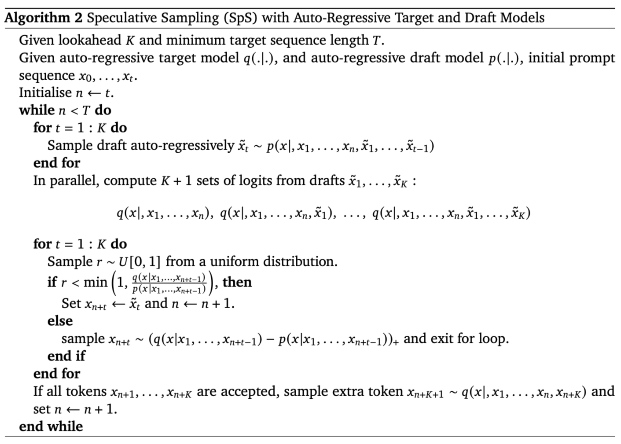
- The draft model decodes K tokens using regular autoregressive methods, producing probability outputs for both the target and draft models on the new predicted sequence.
Token Acceptance Decision:
- By comparing the probabilities from the target and draft models, the algorithm decides how many of the K tokens to retain based on specific rejection criteria. Rejected tokens are resampled using a combination of the two distributions, and further token acceptance is halted.
Final Token Sampling:
- If all K tokens are accepted, an additional final token is sampled from the target model's probability output.
Example:
For instance, with the input "Attention is" and K=3:
The draft model speculates "all you need" (3 tokens).
The target model accepts all and may sample a final token (e.g., a period "."), yielding 4 decoded tokens in a single iteration.
Key Features
Speculative sampling decodes between 1 to K+1 tokens per iteration.
Resampling guarantees the decoding of at least 1 token if no tokens are accepted.
Mathematical equivalence to sampling directly from the target model is maintained.
Seamless integration with existing models without requiring modifications to architecture or training.
Compatible with various inference techniques, including quantization, hardware acceleration, flash attention, and different sampling strategies.
Modified sampling algorithm mentioned in the paper:

Modified Sampling Algorithm (Python Code)
import numpy as np

def sample(p):
    return np.random.choice(np.arange(p.shape[-1]), p=p)

def max_fn(x):
    x_max = np.where(x > 0, x, 0)
    return x_max / np.sum(x_max)

def speculative_sampling(x, draft_model, target_model, N, K):
    # NOTE: paper indexes arrays starting from 1, Python indexes from 0, so
    # we have to add an extra -1 term when indexing using n, T, or t
    n = len(x)
    T = len(x) + N

    while n < T:
        # Step 1: Auto-regressive decode K tokens from draft model and get final p
        x_draft = x
        for _ in range(K):
            p = draft_model(x_draft)
            x_draft = np.append(x_draft, sample(p[-1]))

        # Step 2: Target model forward passes on x_draft
        q = target_model(x_draft)

        # Step 3: Append draft tokens based on rejection criterion and resample
        # a token on rejection
        all_accepted = True
        for _ in range(K):
            i = n - 1
            j = x_draft[i + 1]
            if np.random.random() < min(1, q[i][j] / p[i][j]):  # Accepted
                x = np.append(x, j)
                n += 1
            else:  # Rejected
                x = np.append(x, sample(max_fn(q[i] - p[i])))  # Resample
                n += 1
                all_accepted = False
                break

        # Step 4: If all draft tokens were accepted, sample a final token
        if all_accepted:
            x = np.append(x, sample(q[-1]))
            n += 1

        # Just keeping my sanity
        assert n == len(x), f"{n} {len(x)}"

    return x
The time complexity for this algorithm is given by:
O(N/(r(K+1)) (t_draft * K + t_target)
N/(r(K+1))
Number of iterations in the while loop. It equals the number of tokens to decode (N) divided by the average number of tokens decoded per iteration (r(K+1)). The paper provides the acceptance rate (r), which is the average number of tokens decoded per iteration divided by K+1. Recovering the average number of tokens decoded is achieved by multiplying r by K+1.
t_draft + t_target
Time complexity for each iteration in the loop. The term t_target corresponds to the single forward pass of the target model in step 2, and t_draft * K accounts for the K forward passes of the draft model in step 1.
Modified Sampling Example
Consider two models: M_p (draft model) and M_q (target model). Pf is a prefix string used for sequence completion, and K represents the desired number of tokens to be generated.
Generation Phase
For K=5, the draft model generates tokens in an autoregressive manner:
p1(x) = M_p(pf) -> x1
p2(x) = M_p(pf, x1) -> x2
...
p5(x) = M_p((pf, x1, x2, x3, x4,) -> x5
Target Model Run
Perform a single run of the target model M_q on the sequence pf + x1 + x2 + x3 + x4 + x5
Probability Distributions
Assess probabilities and generate distributions q1(x),q2(x),q3(x),q4(x),q5(x), and q6(x) for all tokens using the target model. These distributions are computed based on the input sequence pf along with the previously generated tokens.
| Token | X1 | X2 | X3 | X4 | X5 |
| dogs | love | chasing | after | cars | |
| p(x) | 0.8 | 0.7 | 0.9 | 0.8 | 0.7 |
| q(x) | 0.9 | 0.8 | 0.8 | 0.3 | 0.8 |
p(x): Probability distribution of the draft model
q(x): Probability distribution of the target model
Note: The table shows probabilities for five words; in reality, there would be distributions for the entire vocabulary.
Rejection sampling of the generated tokens
| Token | X1 | X2 | X3 | X4 | X5 |
| dogs | love | chasing | after | cars | |
| p(x) | 0.8 | 0.7 | 0.9 | 0.8 | 0.7 |
| q(x) | 0.9 | 0.8 | 0.8 | 0.3 | 0.8 |
| q/p ratio | 0.8889 | 0.375 | |||
| Random number generated | 0.4 | 0.5 | |||
| Accepted or Rejected | Accepted | Accepted | Accepted | Rejected | Rejected |
| Reason | Case 1 | Case 1 | Case 2 | Case 3 | Case 4 |
q / p ratio is calculated for each token.
Random numbers are generated for each token.
Decisions (Accepted/Rejected) are made based on the conditions outlined:
Case 1: If q(x) > p(x), then accept.
Case 2: If q(x) < p(x), generate a random number and check if q(x) / p(x) is greater than the random number.
Case 3: All other cases are rejected.
Case 4: Once a previous token is rejected, the rest of the tokens are also dropped.
Adjusted Distribution for Target Model Sampling
Having chosen tokens x1, x2, and x3 from the draft model, the target model comes into play for selecting x4. This is facilitated by leveraging the precomputed probability distribution q4(x).
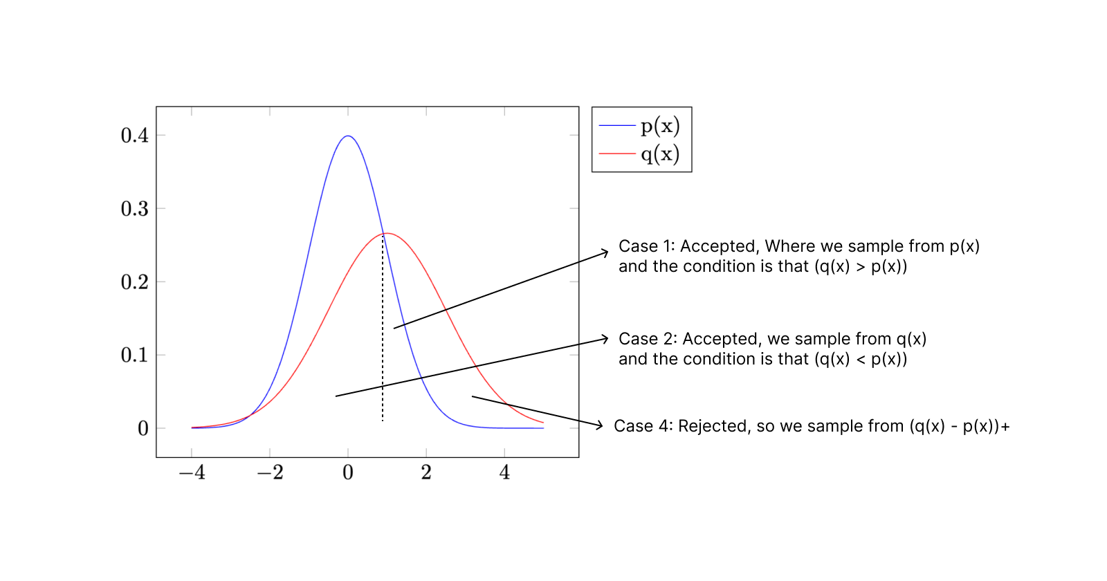
The selection process involves sampling not directly from q(x) but from an adjusted distribution, denoted as (q(x) - p(x))+. Here, the subtraction is performed between token probabilities across the two distributions, with the crucial step of disregarding any parts where the subtraction would yield zero.
The rationale behind this approach is elaborated in Theorem 1 of the paper, and visual clarity is provided through the diagram below.

Upon observation, it becomes apparent that the (q(x) - p(x))+ region in case 4 represents the only remaining area in the q(x) probability distribution after sampling from p(x) in case 1 and q(x) in case 2.
From a logical standpoint, sampling from the (q(x) - p(x))+ region in case 4 ensures that the sampling process for the token distribution collectively aligns with q(x), which is the target model distribution. Therefore, in case 4, the sampling is performed specifically from the (q(x) - p(x))+ region.
How many tokens generated in 1 pass?
Worst case: first token is rejected -> 1 token generated
Best case: all tokens accepted -> K+1 tokens generated
So even in the worst case, we are generating 1 token that is equivalent to Autoregressive sampling. Ultimately this makes speculative sampling at least as good as autoregressive sampling or better.
Results
The paper reports the following speedups for their 70B Chinchilla model (using a specially trained 7B Chinchilla as the draft model):

You can see that there was no performance degradation and the decoding process is 2 times faster as compared to autoregressive decoding.
Let's compare these empirical speedup numbers to theoretical speedup numbers, which we can calculate using our time complexity equations:

Using the values provided in the paper:
K=4
t_draft=1.8ms
t_target=14.1mss
r=0.8 for HumanEval and =0.62 for XSum (see figure 1 in the paper)
For HumanEval we get a theoretical speedup of 2.65, while the paper reports an empirical speedup of 2.46.
For XSum we get a theoretical speedup of 2.05, while the paper reports an empirical speedup of 1.92.
References
Subscribe to my newsletter
Read articles from Aakash Varma directly inside your inbox. Subscribe to the newsletter, and don't miss out.
Written by
Aakash Varma
Aakash Varma
Staff Engineer at kinara.ai I specialise in building advanced compilers for our state-of-the-art edge AI chip. My primary focus revolves around optimising AI models, ensuring they run efficiently and effectively on the chip. I love math, deep learning and optimisation. I dapple in graphic design in my spare time.