Predator->Prey in Python
 Harry Munro
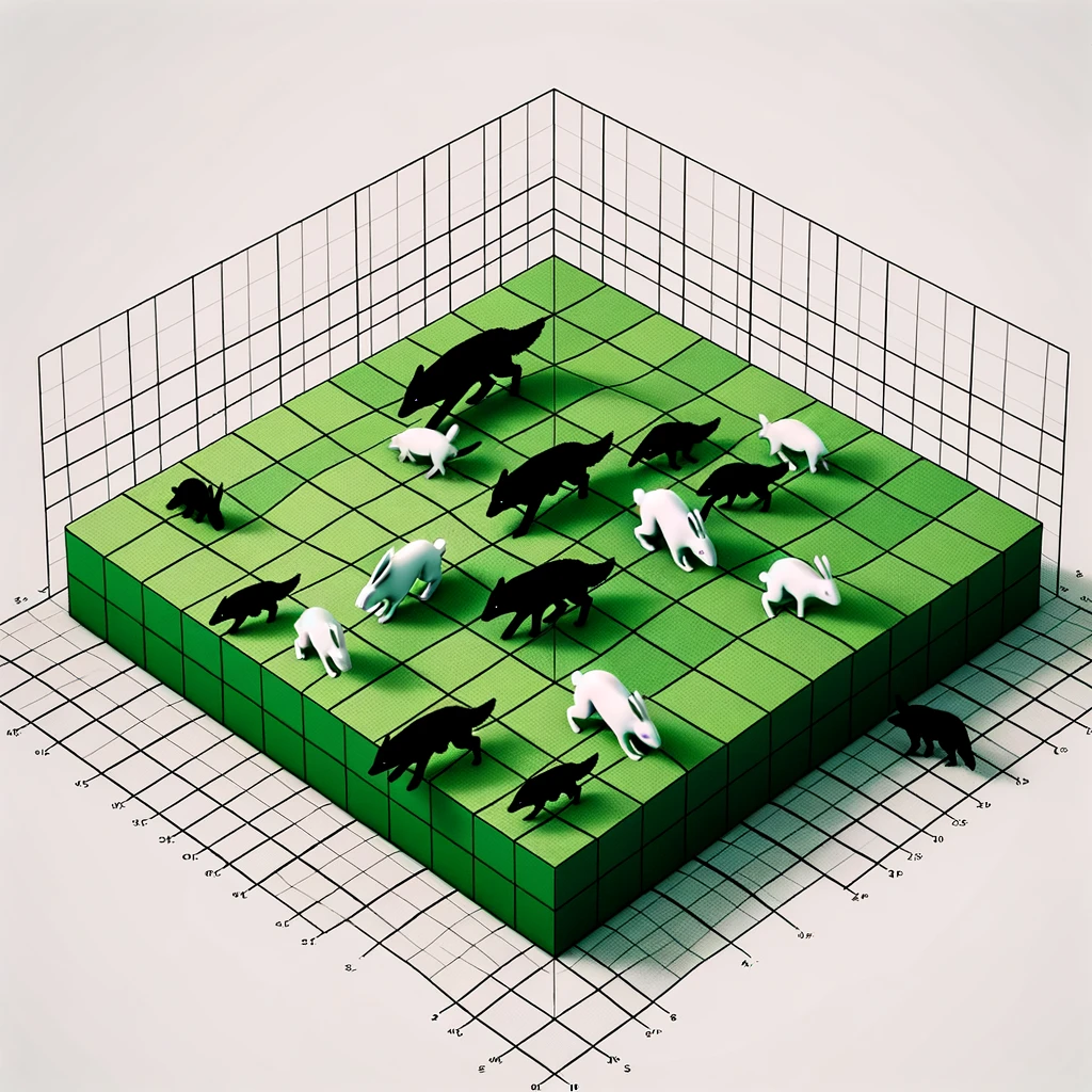
Let's simulate a predator-prey system using agent-based modelling in Python. In this system, we'll have two types of agents: predators (wolves) and prey (rabbits). The rabbits reproduce and are eaten by the wolves, and the wolves must eat to survive and can also reproduce. This system is complex and displays interesting dynamics over time, including oscillations in population sizes.
The key behaviors and rules for our simulation will be:
Rabbits:
Reproduce at a certain rate if there is enough food (grass in their cell).
Move randomly to adjacent cells.
Have a certain chance of being eaten if a wolf is in the same cell.
Wolves:
Move randomly to adjacent cells looking for rabbits.
Eat rabbits to gain energy; if they eat a rabbit, their energy increases, and if they don't eat, their energy decreases.
Reproduce at a certain rate if they have enough energy.
Die if their energy reaches zero.
We'll use a grid to represent the environment where these agents interact. Let's start by setting up the environment and defining the basic behaviors of the rabbits and wolves. Then, we'll run the simulation for a certain number of steps and analyse the population dynamics of both predators and prey using seaborn for visualisation and print key statistics throughout the simulation.
Let's begin by implementing the basic setup and agent behaviors.
import numpy as np
import matplotlib.pyplot as plt
import seaborn as sns

# Parameters
grid_size = 50
initial_rabbits = 100
initial_wolves = 20
rabbit_reproduction_rate = 0.1
wolf_reproduction_rate = 0.1
wolf_energy_gain = 40
initial_wolf_energy = 40
energy_cost = 1
simulation_steps = 1000


# Initial setup
class Cell:
    def __init__(self):
        self.rabbit = False
        self.wolf = False
        self.wolf_energy = 0


# Initialise the grid
grid = np.empty((grid_size, grid_size), dtype=object)
for i in range(grid_size):
    for j in range(grid_size):
        grid[i, j] = Cell()

# Populate the grid
for _ in range(initial_rabbits):
    x, y = np.random.randint(0, grid_size, 2)
    grid[x, y].rabbit = True

for _ in range(initial_wolves):
    x, y = np.random.randint(0, grid_size, 2)
    grid[x, y].wolf = True
    grid[x, y].wolf_energy = initial_wolf_energy


# Function to display grid populations
def display_grid(grid):
    rabbit_grid = np.zeros((grid_size, grid_size))
    wolf_grid = np.zeros((grid_size, grid_size))

    for i in range(grid_size):
        for j in range(grid_size):
            rabbit_grid[i, j] = grid[i, j].rabbit
            wolf_grid[i, j] = grid[i, j].wolf

    fig, ax = plt.subplots(1, 2, figsize=(10, 5))
    sns.heatmap(rabbit_grid, ax=ax[0], cbar=False)
    ax[0].set_title('Rabbits')
    sns.heatmap(wolf_grid, ax=ax[1], cbar=False)
    ax[1].set_title('Wolves')
    plt.show()


# Display initial populations
display_grid(grid)
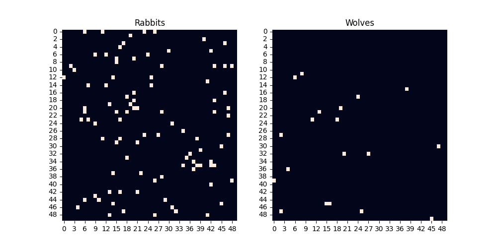
The initial setup of our predator-prey simulation is visualised above, with two grids representing the distribution of rabbits and wolves, respectively, across a 50x50 environment. Rabbits are shown on the left, and wolves are on the right. Each dot represents the presence of an agent in the grid cell.
Next, we will implement the simulation logic, including movement, eating, reproduction, and energy dynamics for wolves and rabbits. After the simulation runs for the specified number of steps, we will analyse the population dynamics and key statistics. Let's proceed with the simulation logic.
def move_agents(grid):
    new_grid = np.empty((grid_size, grid_size), dtype=object)
    for i in range(grid_size):
        for j in range(grid_size):
            new_grid[i, j] = Cell()

    for i in range(grid_size):
        for j in range(grid_size):
            if grid[i, j].rabbit:
                new_i, new_j = (i + np.random.randint(-1, 2)) % grid_size, (j + np.random.randint(-1, 2)) % grid_size
                if not new_grid[new_i, new_j].rabbit:  # Prevent overwriting another rabbit
                    new_grid[new_i, new_j].rabbit = True

            if grid[i, j].wolf:
                new_i, new_j = (i + np.random.randint(-1, 2)) % grid_size, (j + np.random.randint(-1, 2)) % grid_size
                new_grid[new_i, new_j].wolf = True
                new_grid[new_i, new_j].wolf_energy = grid[i, j].wolf_energy  # Transfer energy
                if new_grid[new_i, new_j].rabbit:  # Eat the rabbit
                    new_grid[new_i, new_j].rabbit = False
                    new_grid[new_i, new_j].wolf_energy += wolf_energy_gain
                else:
                    new_grid[new_i, new_j].wolf_energy -= energy_cost  # Energy cost of moving

    return new_grid


def reproduce_agents(grid):
    for i in range(grid_size):
        for j in range(grid_size):
            if grid[i, j].rabbit and np.random.rand() < rabbit_reproduction_rate:
                grid[(i + np.random.randint(-1, 2)) % grid_size, (
                            j + np.random.randint(-1, 2)) % grid_size].rabbit = True

            if grid[i, j].wolf and grid[
                i, j].wolf_energy > initial_wolf_energy and np.random.rand() < wolf_reproduction_rate:
                grid[(i + np.random.randint(-1, 2)) % grid_size, (j + np.random.randint(-1, 2)) % grid_size].wolf = True
                grid[i, j].wolf_energy -= initial_wolf_energy  # Cost of reproduction


def remove_dead_wolves(grid):
    for i in range(grid_size):
        for j in range(grid_size):
            if grid[i, j].wolf and grid[i, j].wolf_energy <= 0:
                grid[i, j].wolf = False


rabbit_counts = []
wolf_counts = []

# Run the simulation
# Re-examining and fixing potential issues in the simulation logic

def simulate_step(grid):
    new_grid = np.empty((grid_size, grid_size), dtype=object)
    for i in range(grid_size):
        for j in range(grid_size):
            new_grid[i, j] = Cell()

    # Move and interact (eat, reproduce) for rabbits and wolves
    for i in range(grid_size):
        for j in range(grid_size):
            cell = grid[i, j]
            if cell.rabbit:
                # Move rabbits
                ri, rj = (i + np.random.randint(-1, 2)) % grid_size, (j + np.random.randint(-1, 2)) % grid_size
                if not new_grid[ri, rj].rabbit:
                    new_grid[ri, rj].rabbit = True
                    # Rabbit reproduction
                    if np.random.rand() < rabbit_reproduction_rate:
                        new_grid[i, j].rabbit = True  # Leave a new rabbit in the original cell

            if cell.wolf:
                # Move wolves
                wi, wj = (i + np.random.randint(-1, 2)) % grid_size, (j + np.random.randint(-1, 2)) % grid_size
                if new_grid[wi, wj].wolf:
                    # If the target cell already has a wolf, try another direction
                    found = False
                    for di, dj in [(-1, 0), (1, 0), (0, -1), (0, 1)]:
                        ni, nj = (wi + di) % grid_size, (wj + dj) % grid_size
                        if not new_grid[ni, nj].wolf:
                            wi, wj = ni, nj
                            found = True
                            break
                    if not found:
                        continue  # Skip moving this wolf if no empty cell is found
                new_grid[wi, wj].wolf = True
                new_grid[wi, wj].wolf_energy = cell.wolf_energy - energy_cost  # Decrease energy for moving

                # Eat rabbit if present
                if new_grid[wi, wj].rabbit:
                    new_grid[wi, wj].rabbit = False
                    new_grid[wi, wj].wolf_energy += wolf_energy_gain

                # Wolf reproduction
                if new_grid[wi, wj].wolf_energy > initial_wolf_energy * 2 and np.random.rand() < wolf_reproduction_rate:
                    new_grid[wi, wj].wolf_energy -= initial_wolf_energy  # Cost of reproduction
                    new_grid[i, j].wolf = True  # Leave a new wolf in the original cell
                    new_grid[i, j].wolf_energy = initial_wolf_energy

    return new_grid


def remove_dead_wolves_fixed(grid):
    for i in range(grid_size):
        for j in range(grid_size):
            if grid[i, j].wolf and grid[i, j].wolf_energy <= 0:
                grid[i, j].wolf = False
                grid[i, j].wolf_energy = 0


# Reset the simulation with the potential fix
grid = np.empty((grid_size, grid_size), dtype=object)
for i in range(grid_size):
    for j in range(grid_size):
        grid[i, j] = Cell()

# Repopulate the grid
for _ in range(initial_rabbits):
    x, y = np.random.randint(0, grid_size, 2)
    grid[x, y].rabbit = True

for _ in range(initial_wolves):
    x, y = np.random.randint(0, grid_size, 2)
    grid[x, y].wolf = True
    grid[x, y].wolf_energy = initial_wolf_energy

# Resetting counts for a fresh simulation
rabbit_counts = []
wolf_counts = []

# Running the simulation with the potential fix
for step in range(simulation_steps):
    grid = simulate_step(grid)  # Use fixed simulation step function
    remove_dead_wolves_fixed(grid)  # Use fixed dead wolf removal function

    rabbit_count = sum(grid[i, j].rabbit for i in range(grid_size) for j in range(grid_size))
    wolf_count = sum(grid[i, j].wolf for i in range(grid_size) for j in range(grid_size))

    rabbit_counts.append(rabbit_count)
    wolf_counts.append(wolf_count)


# Plotting the results
plt.figure(figsize=(10, 5))
plt.plot(rabbit_counts, label='Rabbits')
plt.plot(wolf_counts, label='Wolves')
plt.xlabel('Time Steps')
plt.ylabel('Population')
plt.title('Predator-Prey Population Dynamics')
plt.legend()
plt.show()
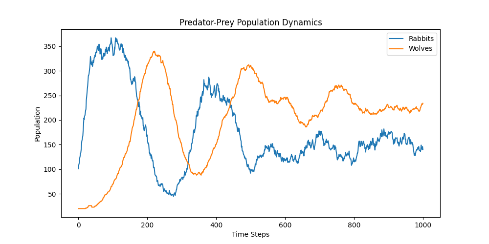
The plot above shows the population dynamics of rabbits and wolves over 1000 simulation steps. As expected in a predator-prey model, we observe oscillations in the populations of both species, with the rabbit population (prey) fluctuating in response to the wolf population (predator) dynamics, and vice versa. Initially, the rabbit population grows, providing more food for wolves, which in turn increases the wolf population. However, as the wolf population grows, it puts pressure on the rabbit population, leading to a decrease in rabbits. This decrease in prey leads to a subsequent decrease in the predator population due to starvation, allowing the rabbit population to recover, and the cycle continues.
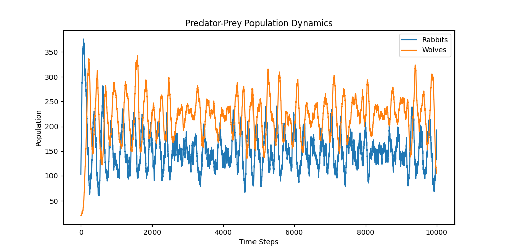
Interestingly we start to see the populations stabilise in our simulation above. Let's extend the simulation now to 10,000 steps (10x as long) and observe what happens to the populations...
To explore and potentially improve the dynamics of the predator-prey simulation, adjusting various parameters can significantly impact the outcome. Here are some key parameters and suggestions on how you might adjust them to observe different behaviors in the simulation:
Reproduction Rates:
Rabbits: Increasing the rabbit reproduction rate might lead to quicker growth of the rabbit population, providing more food for wolves. However, too high a rate could result in an unsustainable explosion of the rabbit population.
Wolves: Adjusting the wolf reproduction rate affects how quickly the wolf population can recover or grow. Be mindful that too high a rate might lead to overpopulation and rapid depletion of the rabbit population.
Energy Dynamics:
Wolf Energy Gain from Eating Rabbits: Increasing the energy wolves gain from eating a rabbit could help sustain the wolf population better, allowing them to reproduce more and survive longer periods without food.
Initial Wolf Energy: Adjusting the initial energy levels of wolves can also impact their survival, especially at the beginning of the simulation.
Energy Cost of Moving: Lowering the energy cost of moving for wolves might help them explore more without facing rapid energy depletion.
Initial Populations: The initial number of rabbits and wolves can set the stage for the simulation's dynamics. A higher initial number of rabbits gives wolves more food sources, while a higher initial number of wolves increases predation pressure on rabbits.
Movement Logic: Though not a parameter, reconsidering the movement logic for both rabbits and wolves could lead to different outcomes. For instance, introducing a more strategic movement for wolves, such as moving towards areas with higher rabbit densities, could make the predator-prey interactions more dynamic.
Simulation Grid Size: The size of the simulation grid affects the density of agents and their interactions. A larger grid might dilute interactions, while a smaller grid could lead to more frequent encounters between rabbits and wolves.
Carrying Capacity for Rabbits: Introducing a carrying capacity (maximum number of rabbits that can be supported by the environment) could prevent the rabbit population from growing indefinitely and promote more cyclical dynamics.
To experiment with these parameters, you can systematically vary one parameter at a time while keeping the others constant to observe its effect on the system's dynamics. This method, known as sensitivity analysis, can help identify which parameters have the most significant impact on the simulation outcome.
Subscribe to my newsletter
Read articles from Harry Munro directly inside your inbox. Subscribe to the newsletter, and don't miss out.
Written by
Harry Munro
Harry Munro
I design, build and test things virtually before decisions are made in the real world.