Refining Realism: Elevating Handwritten Digit Reconstruction with Advanced Generative Models

Greetings, readers,

This article follows on from my prior exploration of reconstructing handwritten digits titled “Crafting Realism: A Journey into Handwritten Digit Reconstruction with Stacked Autoencoders ,GANs, and Deep Convolutional GANs”, In this installment, we delve into the realm of diffusion models for the same purpose.

Prior to examining the implementation, let's first grasp the concept of a diffusion model and understand what diffusion entails.

Diffusion Models are generative models, meaning that they are used to generate data similar to the data on which they are trained. Fundamentally, Diffusion Models work by destroying training data through the successive addition of Gaussian noise and then learning to recover the data by reversing this noising process. After training, we can use the Diffusion Model to generate data by simply passing randomly sampled noise through the learned denoising process. It is inspired from thermodynamics to model a diffusion process, similar to a drop of milk diffusing in a cup of tea. The core idea is to train a model to learn the reverse process: start from the completely mixed state, and gradually "unmix" the milk from the tea.

Kindly refer [2006.11239v2] Denoising Diffusion Probabilistic Models (arxiv.org) for a detailed explanation. DDPMs (Denoising Diffusion Probabilistic Models) are much easier to train than GANs, and the generated images are more diverse and of even higher quality. The downside of DDPMs is that they take a very long time to generate images, unlike GANs or VAEs.

Code Implementation:

import warnings
warnings.filterwarnings('ignore')
import matplotlib.pyplot as plt
import numpy as np
import tensorflow as tf

mnist = tf.keras.datasets.mnist.load_data()
(X_train_full, y_train_full), (X_test, y_test) = mnist
X_train_full = X_train_full.astype(np.float32) / 255

from sklearn.model_selection import train_test_split

X_train, X_valid, y_train, y_valid = train_test_split(X_train_full, y_train_full, test_size=0.2, random_state=42)

Forward Process:

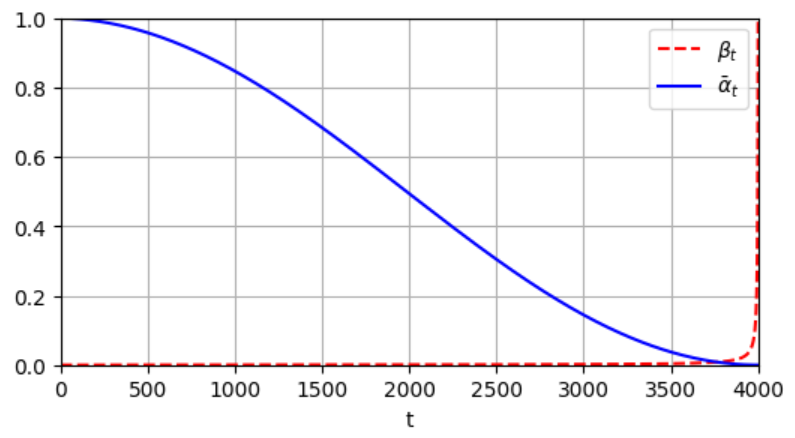
So how exactly does a DDPM work? let's take a picture of a cat and at each time step t and you add a little bit of Gaussian noise to the image, with mean 0 and variance β. The noise is independent for each pixel. We continue this process until the cat is completely hidden by the noise, impossible to see. The last time is noted T. The variance is scheduled in such a way that the cat signal fades linearly between the time steps 0 and T. This is called the forward process.

Variance Schedule equations:

In these equations :

• s is a tiny value that prevents β_t from being too small near t=0.

• β_t is clipped to be no longer than 0.999, to avoid instabilities near t=T.

def variance_schedule(T, s=0.008, max_beta=0.999):
    t = np.arange(T + 1)
    f = np.cos((t / T + s) / (1 + s) * np.pi / 2) ** 2
    alpha = np.clip(f[1:] / f[:-1], 1 - max_beta, 1)
    alpha = np.append(1, alpha).astype(np.float32)  # add α₀ = 1
    beta = 1 - alpha
    alpha_cumprod = np.cumprod(alpha)
    return alpha, alpha_cumprod, beta  # αₜ , α̅ₜ , βₜ for t = 0 to T

np.random.seed(42) 
T = 4000
alpha, alpha_cumprod, beta = variance_schedule(T)

Here we take T = 4000, as per the Improved DDPM paper.

Reverse Process:

To train our model to reverse the diffusion process, we will need noisy images from different steps of the forward process.

def prepare_batch(X):
    X = tf.cast(X[..., tf.newaxis], tf.float32) * 2 - 1  # scale from –1 to +1
    X_shape = tf.shape(X)
    t = tf.random.uniform([X_shape[0]], minval=1, maxval=T + 1, dtype=tf.int32)
    alpha_cm = tf.gather(alpha_cumprod, t)
    alpha_cm = tf.reshape(alpha_cm, [X_shape[0]] + [1] * (len(X_shape) - 1))
    noise = tf.random.normal(X_shape)
    return {
        "X_noisy": alpha_cm ** 0.5 * X + (1 - alpha_cm) ** 0.5 * noise,
        "time": t,
    }, noise

def prepare_dataset(X, batch_size=32, shuffle=False):
    ds = tf.data.Dataset.from_tensor_slices(X)
    if shuffle:
        ds = ds.shuffle(10_000)
    return ds.batch(batch_size).map(prepare_batch).prefetch(1)

tf.random.set_seed(43) 
train_set = prepare_dataset(X_train, batch_size=32, shuffle=True)
valid_set = prepare_dataset(X_valid, batch_size=32)

def subtract_noise(X_noisy, time, noise):
    X_shape = tf.shape(X_noisy)
    alpha_cm = tf.gather(alpha_cumprod, time)
    alpha_cm = tf.reshape(alpha_cm, [X_shape[0]] + [1] * (len(X_shape) - 1))
    return (X_noisy - (1 - alpha_cm) ** 0.5 * noise) / alpha_cm ** 0.5

X_dict, Y_noise = list(train_set.take(1))[0]  # get the first batch
X_original = subtract_noise(X_dict["X_noisy"], X_dict["time"], Y_noise)

Our goal is not to drown the cats in noise. On the contrary, we want to create many new cats! So we need to build a model that can perform the reverse process: going from x_t to x_t-1. We can use this to remove a tiny bit of noise from an image at each step, and gradually remove all noise from the image.

Building the diffusion model:

embed_size = 64

class TimeEncoding(tf.keras.layers.Layer):
    def __init__(self, T, embed_size, dtype=tf.float32, **kwargs):
        super().__init__(dtype=dtype, **kwargs)
        assert embed_size % 2 == 0, "embed_size must be even"
        p, i = np.meshgrid(np.arange(T + 1), 2 * np.arange(embed_size // 2))
        t_emb = np.empty((T + 1, embed_size))
        t_emb[:, ::2] = np.sin(p / 10_000 ** (i / embed_size)).T
        t_emb[:, 1::2] = np.cos(p / 10_000 ** (i / embed_size)).T
        self.time_encodings = tf.constant(t_emb.astype(self.dtype))

    def call(self, inputs):
        return tf.gather(self.time_encodings, inputs)

def build_diffusion_model():
    X_noisy = tf.keras.layers.Input(shape=[28, 28, 1], name="X_noisy")
    time_input = tf.keras.layers.Input(shape=[], dtype=tf.int32, name="time")
    time_enc = TimeEncoding(T, embed_size)(time_input)

    dim = 16
    Z = tf.keras.layers.ZeroPadding2D((3, 3))(X_noisy)
    Z = tf.keras.layers.Conv2D(dim, 3)(Z)
    Z = tf.keras.layers.BatchNormalization()(Z)
    Z = tf.keras.layers.Activation("relu")(Z)

    time = tf.keras.layers.Dense(dim)(time_enc)  # adapt time encoding
    Z = time[:, tf.newaxis, tf.newaxis, :] + Z  # add time data to every pixel

    skip = Z
    cross_skips = []  # skip connections across the down & up parts of the UNet

    for dim in (32, 64, 128):
        Z = tf.keras.layers.Activation("relu")(Z)
        Z = tf.keras.layers.SeparableConv2D(dim, 3, padding="same")(Z)
        Z = tf.keras.layers.BatchNormalization()(Z)

        Z = tf.keras.layers.Activation("relu")(Z)
        Z = tf.keras.layers.SeparableConv2D(dim, 3, padding="same")(Z)
        Z = tf.keras.layers.BatchNormalization()(Z)

        cross_skips.append(Z)
        Z = tf.keras.layers.MaxPooling2D(3, strides=2, padding="same")(Z)
        skip_link = tf.keras.layers.Conv2D(dim, 1, strides=2,
                                           padding="same")(skip)
        Z = tf.keras.layers.add([Z, skip_link])

        time = tf.keras.layers.Dense(dim)(time_enc)
        Z = time[:, tf.newaxis, tf.newaxis, :] + Z
        skip = Z

    for dim in (64, 32, 16):
        Z = tf.keras.layers.Activation("relu")(Z)
        Z = tf.keras.layers.Conv2DTranspose(dim, 3, padding="same")(Z)
        Z = tf.keras.layers.BatchNormalization()(Z)

        Z = tf.keras.layers.Activation("relu")(Z)
        Z = tf.keras.layers.Conv2DTranspose(dim, 3, padding="same")(Z)
        Z = tf.keras.layers.BatchNormalization()(Z)

        Z = tf.keras.layers.UpSampling2D(2)(Z)

        skip_link = tf.keras.layers.UpSampling2D(2)(skip)
        skip_link = tf.keras.layers.Conv2D(dim, 1, padding="same")(skip_link)
        Z = tf.keras.layers.add([Z, skip_link])

        time = tf.keras.layers.Dense(dim)(time_enc)
        Z = time[:, tf.newaxis, tf.newaxis, :] + Z
        Z = tf.keras.layers.concatenate([Z, cross_skips.pop()], axis=-1)
        skip = Z

    outputs = tf.keras.layers.Conv2D(1, 3, padding="same")(Z)[:, 2:-2, 2:-2]
    return tf.keras.Model(inputs=[X_noisy, time_input], outputs=[outputs])

The DDPM authors used a modified U-Net architecture which is very similar to FCN architecture. Going one step is described by the following equation:

tf.random.set_seed(42) 
model = build_diffusion_model()
model.compile(loss=tf.keras.losses.Huber(), optimizer="nadam")

# extra code – adds a ModelCheckpoint callback
checkpoint_cb = tf.keras.callbacks.ModelCheckpoint("my_diffusion_model.keras",
                                                   save_best_only=True)

history = model.fit(train_set, validation_data=valid_set, epochs=100,
                    callbacks=[checkpoint_cb])

def generate(model, batch_size=32):
    X = tf.random.normal([batch_size, 28, 28, 1])
    for t in range(T - 1, 0, -1):
        print(f"\rt = {t}", end=" ")  # extra code – show progress
        noise = (tf.random.normal if t > 1 else tf.zeros)(tf.shape(X))
        X_noise = model({"X_noisy": X, "time": tf.constant([t] * batch_size)})
        X = (
            1 / alpha[t] ** 0.5
            * (X - beta[t] / (1 - alpha_cumprod[t]) ** 0.5 * X_noise)
            + (1 - alpha[t]) ** 0.5 * noise
        )
    return X

tf.random.set_seed(42)
X_gen = generate(model)

Results:

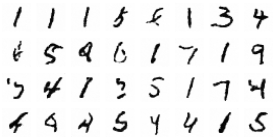
In summary, the investigation into diffusion models for reconstructing handwritten digits reveals a promising avenue in generative modeling. These models utilize a technique of gradually introducing and then reversing Gaussian noise, proving effective in generating data resembling the training dataset. With ongoing research and improvements, diffusion models offer potential contributions to various applications, including image generation and data augmentation. As we delve further into generative modeling, the development of diffusion models showcases innovation within the field and sets the stage for further advancements and breakthroughs. feel free to check out the Source code: avd1729/Diffusion (github.com)