Fourier Transformations for Images

Introduction

In the vast realms of digital image processing, few tools wield as much power and influence as the Fourier Transform. It serves as a cornerstone for unraveling the intricate frequency makeup of images, enabling us to peer into their underlying structures with unprecedented clarity. Yet, for many, the Fourier Transform remains shrouded in mystery, its inner workings seemingly arcane and complex.

In this blog, we embark on a journey to understand the Fourier Transform in the context of image processing. We will strip away the layers of abstraction, breaking down its principles into digestible concepts, and guide you through a hands-on Python implementation from scratch. By the end of this exploration, you'll not only grasp the essence of Fourier Transform but also wield the tools to harness its transformative power in your own projects.

Understanding Fourier Transform

At its core, the Fourier Transform is a mathematical tool that enables us to decompose complex function into its constituent frequencies. In the context of image processing, it allows us to analyze an image in terms of the spatial frequency present with it.

Mathematically, the 1D Fourier Transform of a continuous function \(f(x)\) is defined as

\[F(u) = \int_{-\infty}^{\infty} f(x) e^{-i2\pi ux}dx\]

Here, \(F(u)\) represents the frequency domain representation of the function \(f(x)\), and \(u\) denotes the frequency variable. The term \(e^{-i2\pi ux}\) corresponds to the complex sinusoidal waves with varying frequencies.

Extending to 2D images, we have the Fourier Transform represented as:

\[F(u, v) = \int\int_{-\infty}^{\infty}f(x, y)e^{-i2\pi (ux + vy)} dxdy\]

In the context of images, \(f(x, y)\) represents the intensity values at each pixel coordinate \((x, y)\), and \(F(u, v)\) represents the frequency domain representation of the image.

The Fourier Transform essentially expresses the image as sum of sinusoidal waves of different frequencies and orientations. Low frequencies represent smooth transitions in the image, while high frequencies capture rapid changes, such as edges and textures. Understanding this decomposition is pivotal for various image processing tasks, from denoising to feature extraction.

Preparing the Image

Before diving into Fourier Transform, it's crucial to prepare the image for analysis. In the digital realm, images are represented as matrices of pixel intensities. Thus, we must ensure our image is in a suitable format for preprocessing.

Firstly, we may need to resize the image to a manageable size, balancing computational efficiency with preserving important details. Additionally, converting the image into grayscale simplifies the analysis by removing color complexity.

Furthermore, ensuring that the dimensions of the image are compatible with Fourier Transform operation is essential. For efficient computation and interpretation, it's often beneficial to work with images whose dimensions are powers of 2.

By performing these preprocessing steps, we lay the groundwork for accurate and efficient Fourier Transform analysis, setting the stage for deeper insights into the frequency makeup of the image.

Implementing Fourier Transform in Python

Now, lets dive into the implementation of Fourier Transform in Python. We will start with the 1D Fourier Transform and then extend it to 2D images. Below is a step-by-step explanation of the code:

import numpy as np
import matplotlib.pyplot as plt

def discrete_fourier_transform(signal):
    N = len(signal)
    frequencies = np.arange(N)
    spectrum = np.zeros(N, dtype=np.complex)

    for k in range(N):
        spectrum[k] = np.sum(signal * np.exp(-2j * np.pi * k * frequencies / N))

    return spectrum

# Generating a composite signal
t = np.linspace(0, 1, 1000)
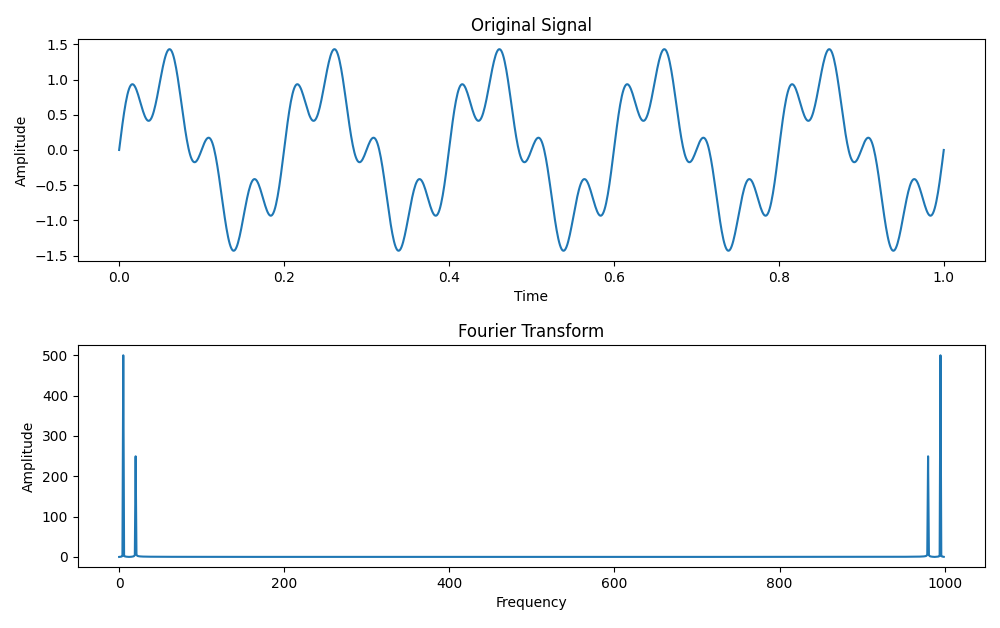
signal = np.sin(2 * np.pi * 5 * t) + 0.5 * np.sin(2 * np.pi * 20 * t)

# Performing Fourier Transform
spectrum = discrete_fourier_transform(signal)

# Plotting the original signal and its Fourier Transform
plt.figure(figsize=(10, 6))
plt.subplot(2, 1, 1)
plt.plot(t, signal)
plt.title("Original Signal")
plt.xlabel("Time")
plt.ylabel("Amplitude")

plt.subplot(2, 1, 2)
plt.plot(np.abs(spectrum))
plt.title("Fourier Transform")
plt.xlabel("Frequency")
plt.ylabel("Amplitude")

plt.tight_layout()
plt.show()

The frequency decomposition looks as follows:

Having grasped the essence of 1D Fourier Transform, let's now extend our exploration to 2D, applying it to images. The principles remain the same, but we will be operating on a two-dimensional grid of pixel intensities instead of one-dimensional signal.

import numpy as np
import matplotlib.pyplot as plt

def discrete_fourier_transform_2D(image):
    M, N = image.shape
    spectrum = np.zeros((M, N), dtype=np.complex)

    for u in range(M):
        for v in range(N):
            for x in range(M):
                for y in range(N):
                    spectrum[u, v] += image[x, y] * np.exp(-2j * np.pi * ((u * x) / M + (v * y) / N))

    return spectrum

# Load and preprocess the image
image = plt.imread("image.jpg")
image_gray = np.mean(image, axis=2)  # Convert to grayscale

# Performing 2D Fourier Transform
spectrum_2d = discrete_fourier_transform_2D(image_gray)

# Plotting the original image and its Fourier Transform
plt.figure(figsize=(18, 6))
plt.subplot(1, 3, 1)
plt.imshow(image_gray, cmap="gray")
plt.title("Original Image")
plt.axis("off")

plt.subplot(1, 3, 2)
plt.imshow(np.abs(spectrum_2d), cmap="gray")
plt.title("2D Fourier Transform")
plt.axis("off")

plt.subplot(1, 3, 3)
plt.imshow(np.log(1 + np.abs(spectrum_2d)), cmap="gray")
plt.title("Shifted 2D Fourier Transform")
plt.axis("off")

plt.tight_layout()
plt.show()

However, the above code, while correct in essence, suffers from a significant drawback: it is painfully slow. The nested loops used to compare the 2D Fourier Transform result in a time complexity of \(O(M^2N^2)\), where \(M\) and \(N\) represent the dimensions of the image. This biquadratic time (when \(M=N\)) complexity becomes prohibitively slow for larger images, hindering its practical utility in real-world applications.

To address this issue, we turn to Fast-Fourier Transform (FFT) algorithm, a technique that drastically reduces the the complexity of Fourier Transform from \(O(N^2) \) to \(O(NlogN)\), making it feasible for processing large datasets in reasonable timeframes.

The Fast Fourier Transform algorithm is a sophisticated technique for computing the Discrete Fourier Transform with significantly reduced time complexity. At its core, FFT exploits the inherent symmetries and periodicities in the Fourier Transform to efficiently compute the frequency domain representation of a signal or image.

The FFT algorithm operates by recursively dividing the DFT computation into smaller subproblems. It leverages a divide-and-conquer approach to efficiently compute the frequency domain representation in \(O(NlogN)\) time complexity.

At each stage of the recursion, the FFT algorithm splits the signal into even and odd components, computes their FFTs separately, and combines them using the FFT butterfly operation. This process effectively reduces the computational complexity by exploiting the inherent structure of the Fourier Transform.

Now let's delve into implementing the FFT from scratch using NumPy:

import numpy as np
import matplotlib.pyplot as plt

def fft(signal):
    N = len(signal)
    if N <= 1:
        return signal
    even = fft(signal[::2])
    odd = fft(signal[1::2])
    factor = np.exp(-2j * np.pi * np.arange(N) / N)
    return np.concatenate([even + factor[:N // 2] * odd, even + factor[N // 2:] * odd])

def fft_2D(image):
    M, N = image.shape
    spectrum = np.zeros((M, N), dtype=np.complex)

    for i in range(M):
        spectrum[i, :] = fft(image[i, :])
    for j in range(N):
        spectrum[:, j] = fft(spectrum[:, j])

    return spectrum

# Load and preprocess the image (image_gray)
image = plt.imread("image.jpg")
image_gray = np.mean(image, axis=-1)
spectrum_2d_fft = fft_2D(image_gray)

# Plotting the original image and its Fourier Transform using FFT
plt.figure(figsize=(12, 6))
plt.subplot(1, 2, 1)
plt.imshow(image_gray, cmap="gray")
plt.title("Original Image")
plt.axis("off")

plt.subplot(1, 2, 2)
plt.imshow(np.log(1 + np.abs(spectrum_2d_fft)), cmap="gray")
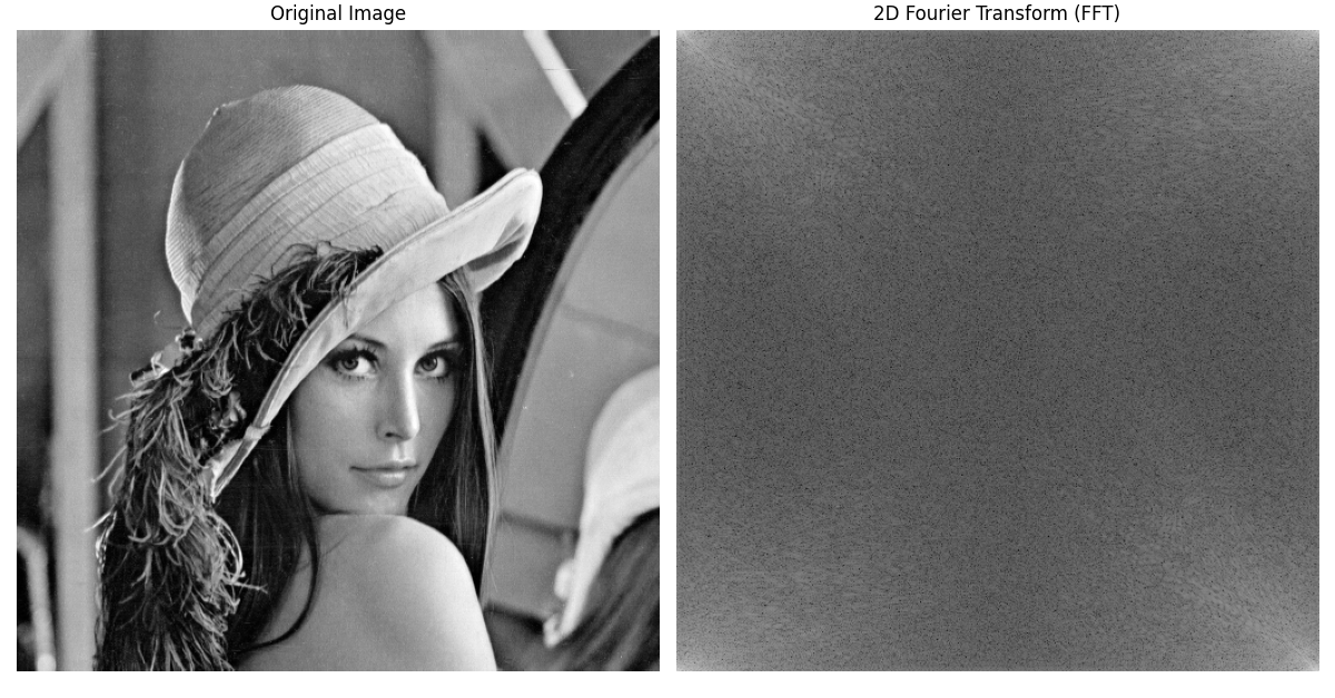
plt.title("2D Fourier Transform (FFT)")
plt.axis("off")

plt.tight_layout()
plt.show()

Are we done with the Fourier Transforms? Not yet. While we have successfully computed the Fourier Transform of our image, there is one crucial step left: understanding the DC component in the frequency domain and ensuring proper visualization. The DC Component represents the zero-frequency term, corresponding to the average intensity of the image.

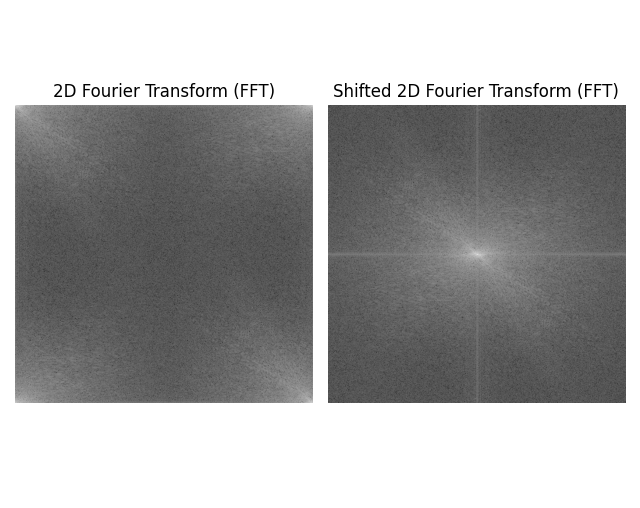
In the frequency domain representation of the image, the DC component is located at the center of the spectrum. However, when plotting the spectrum we often prefer to visualize it with the DC component at the top-left corner for better interpretability. This is where the Fourier Shift operation comes into play. It shifts the zero-frequency domain to the center of the spectrum, making it easier to analyze and interpret the frequency content of the image.

Let's implement the this operation from scratch

def fftshift(spectrum):
    M, N = spectrum.shape
    shift_spectrum = np.zeros_like(spectrum)

    shift_spectrum[:M//2, :N//2] = spectrum[M//2:, N//2:]
    shift_spectrum[:M//2, N//2:] = spectrum[M//2:, :N//2]
    shift_spectrum[M//2:, :N//2] = spectrum[:M//2, N//2:]
    shift_spectrum[M//2:, N//2:] = spectrum[:M//2, :N//2]

    return shift_spectrum

This shift can be visualized as follows:

Since the blog has gone too heavy on concepts and programming, let's continue it in the next one. Stay tuned for the next blog!