A Railroad Simulation with DES
 Mia Temma
In our previous post, we introduced how to utilize Discrete Event Simulation (DES) in PicoLisp. Now, let's explore another application: a railroad model simulation that includes tracks and trains. The visualization is ASCII-based, so feel free to unleash your imagination to transform it into a comprehensive mini railway experience! 😊
You can create a sort of "model of a model railroad" with the program, and it serves no other purpose than having fun.
The sources can be found on GitLab or downloaded from https://software-lab.de/bahn.tgz (source code within the "misc/"-folder). PicoLisp version >= 23.12 is required.
Concept
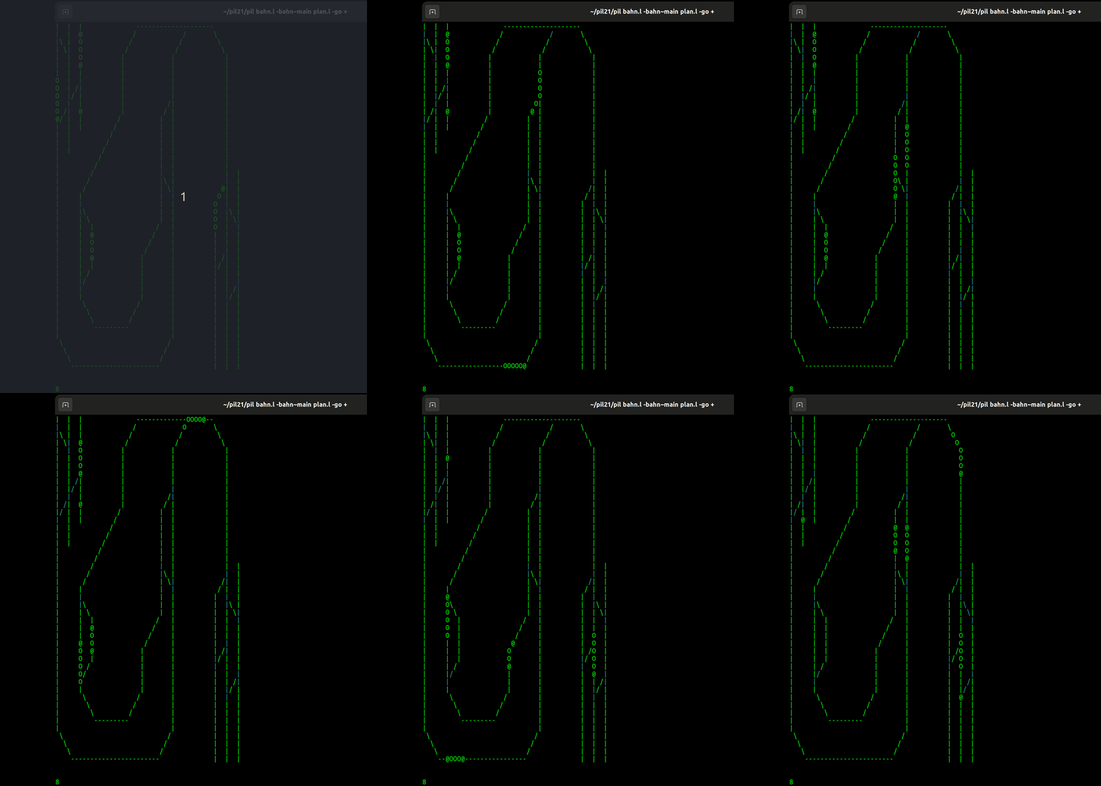
The base of the simulation is a railroad network drawn in ASCII, with each line representing a track. The cyan lines represent switches that enable the trains to change tracks.
The trains are the simulated objects ("bots"). They are depicted as @000 , where the @ mark represents the locomotive and each 0 represents a wagon.
At any point in time, a train is either
waiting, e.g. at a station,
moving from one position to another,
or shunting (rearranging locomotive and wagons).
Let's see it in action in the example below. There are 5 trains in operation - some with multiple wagons, some with a locomotive at each end, and one solitary locomotive without any wagons.
For each train an individual schedule has been defined based on a specified order of positions. However, the precise movements of the trains are determined dynamically using Discrete Event Simulation.
The GIF below is showing the first 30 seconds of the simulation running at 8x speed.

Running the simulation
The source code is split into two files:
bahn.l, containing the fundamental logic for the train and network simulation.plan.l, containing the railway network layout and driving parameters, such as the number and specifications of trains, schedule, speed, etc.
Note: if you are confused about the wording - "bahn" is the German word for train :)
To start the simulation, use the following command:
$ pil bahn.l -bahn~main plan.l -go +
Typing "s" starts and stops the simulation, while the simulation speed doubles and halves with "+" and "-" respectively. ESC will drop you into the REPL, and calling (go) from the REPL will continue with the simulation. To exit the simulation, press ESC and then Ctrl-D or (bye).
Train Simulation in Detail
A train can be in three states: Waiting, moving and shunting.
Waiting is realized using the pause function of the DES library.
More interesting is moving, which consists of several steps:
Acceleration until reaching travel speed.
Continuous travel at the designated speed.
Deceleration upon reaching the destination.
Discrete Event Simulation offers several advantages over continuous simulation, particularly when dealing with numerous bots with varying timings. For instance, continuous simulation will use a fixed time slice dt and the bot's current speed v to calculate their change in position, using the following differential equation:

This calculation is performed for all bots, regardless of their individual speeds.
In contrast, discrete event simulation utilizes a spatial resolution ds (which may vary for each bot and scenario) and computes the time required to "pause" in the simulation until the bot has covered the distance:

Now, all moving bots remain inactive for their scheduled amounts of time - longer if they move at slower speeds and/or coarser resolutions. This approach can significantly reduce processing time.
Note that the equations above are valid only for moving at constant speed. For accelerated movement, a continuous simulation would calculate:

For discrete event simulation, we can use:

This behavior is implemented in the drive function in the file bahn.l. The function takes the following parameters: acceleration (in m/s², also utilized for deceleration during braking), travel speed (in m/s), and X and Y coordinates for the destination. Optionally, additional X and Y destination pairs can be provided to enforce intermediate stops.
For each destination, the function searches for a viable path through the track network and attempts to lock the path. If the path is unavailable, it enters a pause state until receiving a signal that another bot has released the locks. It also toggles all necessary switches as required for its route.
Now the last train state, shunting, which is implemented in the shunt function in bahn.l. This function disconnects the locomotive from the first wagon, calls drive and turn repeatedly to navigate to the other end of the train, and connects to the previously last wagon.
As an example, this is how the first locomotive is defined in bahn.l.
(new '(+Locomotive) (pd 1 10 'a) 5
   (pause)
   (loop
      (drive 0.2 40.0  31 14)
      (pause 12.0)
      (drive 0.2 40.0  45 34)
      (shunt
         (drive 0.1 10.0  45 38)
         (turn)
         (drive 0.1 10.0  48 32  45 23)
         (turn)
         (drive 0.1 10.0  45 28) )
      (drive 0.2 40.0  31 19)
      ...  ) ) )
The pd method of the locomotive object defines that the locomotive starts at position (x, y) = (1, 10) and faces in direction of a, e. g. downwards. The last parameter of the first line, 5, indicates the number of wagons.
As mentioned above, the drive method takes four parameters: acceleration, speed, and a target x-y-position. drive is also used within the shunt method to define the movement of the locomotive while the wagons stay at their current position.
With this, we have covered all possible states of the train. Next we will see how the track network is implemented.
Track Simulation in Detail
For the railway tracks to run the trains on, we use the track network library available in the PicoLisp distribution. The library has a tracks function in @lib/simul.l, which processes the ASCII representation of a railway layout from the current input stream and generates an appropriate data structure.
The idea is to have interconnected track elements where the bots can be positioned, along with a cdr-like operation to move a bot from one element to the next. Iterating this operation results in a continuous movement into one direction.
However, for a comprehensive track network, a simple linked list of track elements is insufficient. It must be possible to traverse it in both directions and accommodate switches (turnouts) and loops. Loops present a particular challenge. Consider this layout where a bot starts in the top-right position and moves leftwards:
             <--               <--
       ---------------------------------
      /                 /      -->
     /                 /
    /                 /
   |                 |
   |                 |
   |                 |
    \               /
     \             /
      \           /
       -----------
           -->
After traversing the loop, it ends up in the top-right position again, but now moving in the opposite direction! The cdr operation would throw it back into the loop instead of continuing in the intended direction.
To address this, the tracks function generates what we call a "Networked Linked Lists" data structure. This structure is a form of indirect doubly linked list that accommodates branches, allowing for traversal in both directions and supporting complex track layouts such as loops.
The structure can be visualized with the built-in ASCII diagramming capabilities of the PicoLisp Vip editor. In the PicoLisp REPL (in debug mode!) enter
: (vi "@doc/Tracks")
and type "v" to view it in a new buffer. It will show:
Connectors:

---------+                 +------------->   +----------------------------->
         |                 |                 |
         v                 |                 |
      +-----+-----+     +--+--+-----+     +--+--+-----+
  +-->|  |  |  ---+---->|  |  |  ---+---->|  |  |  |  |
  |   +--+--+-----+     +-----+-----+     +-----+--+--+
  |      | ^                                       |
  |      | |                                       |
  |      | +---------------------------------------|-----------------+
  |      |                                         |                 |
  |      |                                         |                 |
  |      |      +----------+ +---------------------+                 |
  |      |      |          | |                                       |
  |      v      v          | v                                       |
  |   +------------+    +--+--+-----+     +-----+-----+     +-----+--+--+
  +---+- a      b -+--->|  |  |  ---+---->|  |  |  ---+---->|  |  |  |  |
      |            |    +-----+-----+     +--+--+-----+     +--+--+-----+
      |   Track    |       ^                 |                 |
      |            |       |                 |                 |
      | x        y |       +-----------------|-----------------|------------
      +------------+                         |                 |
                                             |                 |
<--------------------------------------------+   <-------------+
As you can see, it is a rather complicated structure. The Track box is a symbol holding the actual track element. It stores information like the x and y coordinates and connectors to the neighboring track elements in a and b. Each connector consists of three cells for forward- and backward-links and optional switches in both directions.
User Interface
Showing the animated ASCII drawing and handling user keyboard input is all done by a single function called display. It is called by go in a loop until ESC is typed, and allows to move around in the layout or along a rail track, and to toggle switches manually. Additionally, the following commands can be used in order to interact with the simulation:
sstops or continues the simulation.+and-double and halve the simulation speed respectively. Initially, the speed factor is 2. It is displayed at the bottom left.A red `#` cursor (initially hidden on the left outside the layout) can be moved around on the screen with the following keystrokes:
jorDOWN,korUP,landhmove by a single positionzandZmove by eight positions right and leftwandbmove by a "word" (e.g. rail element) to the right and left0and$to go to left and right end of the layoutgandGgo to top and bottom of the layoutTABandBACKto jump to the next and previous switchENTERto toggle a switchSPACEto move along the trackrto toggle the move direction for theSPACEcommand.
Now, with this information you should have a good understanding of how to create a railway model using discrete event simulation in PicoLisp. By referring to the examples on GitLab, tweaking it into your own railway model shouldn't be too challenging.
With some (considerable) effort, you could even replace the ASCII representation by something more visually appealing 😊

Sources
Subscribe to my newsletter
Read articles from Mia Temma directly inside your inbox. Subscribe to the newsletter, and don't miss out.
Written by
