TinyML (Part 2)

Minimizing loss with Gradiant descent

Assume this is our loss function

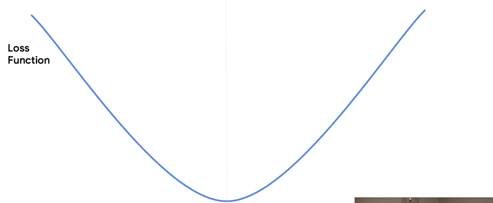
If we want to know the minimum of the loss function, we just look to the bottom of the parabola. It doesn't matter whatever the parameters that make up the function are and wherever this would be plotted on a chart. We will still know that the minimum is at the bottom.

So if we made a guess as to what the parameters of our equation would be-- say we had started with y equals 10x plus 10, for example-- and we calculated the loss for the data in our equation, we know that it would be very high and so very far away from the minimum. Maybe it would look a little bit like this. Now it gets interesting. And here's why you generally see a lot of math and calculus in machine learning.

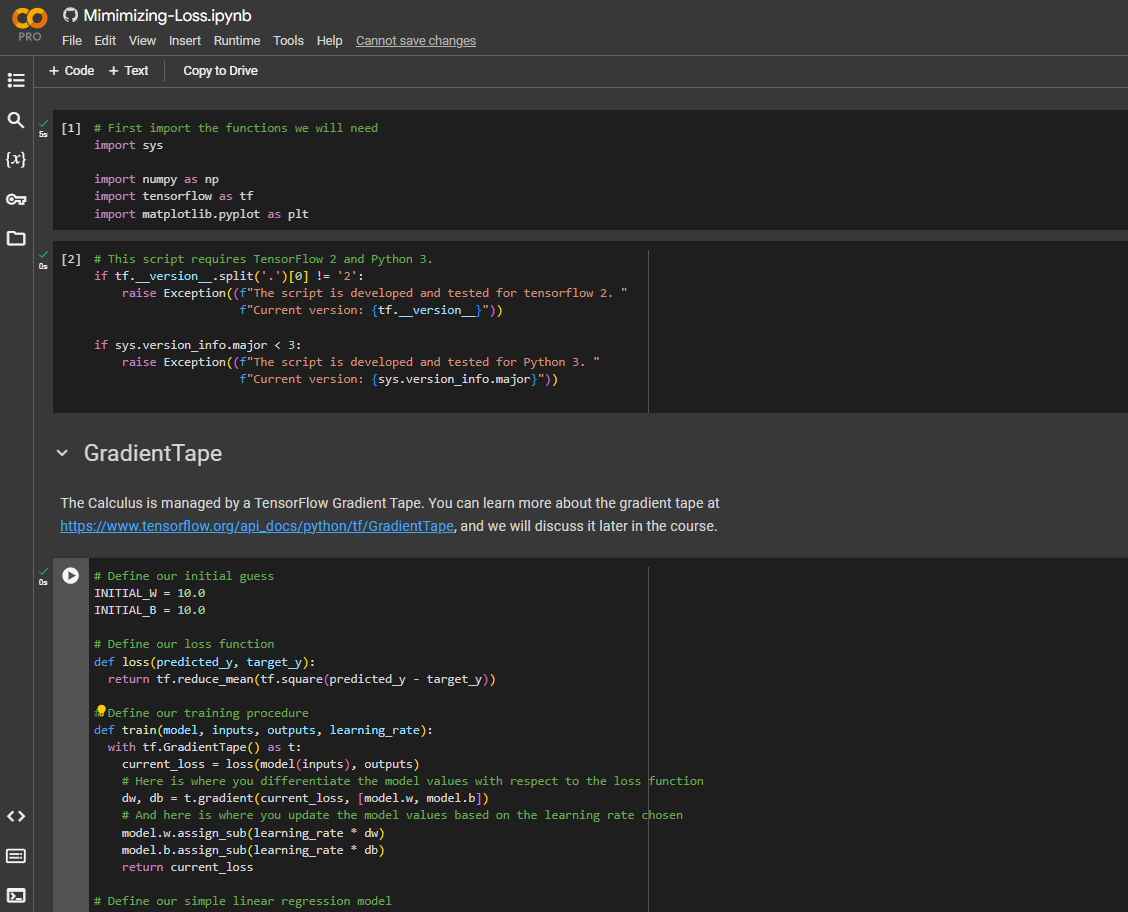
If you differentiate the values with respect to the loss function, you'll get a gradient.

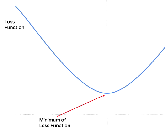
With gradiant you can know the direction of the bottom

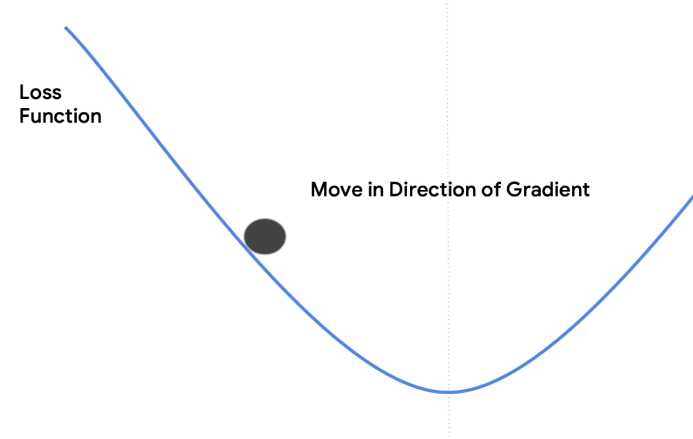
The nice thing about having a gradient is that you can use it to determine the direction towards the bottom. It's actually the negative of the gradient points that way. You have no idea how far it is to the bottom, but at least you know the correct direction. It's like a ball on a slope.

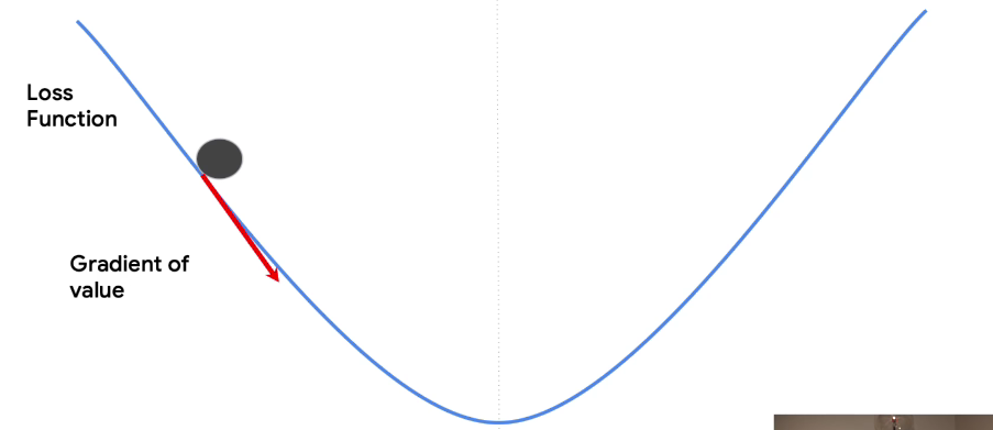
Gravity will give you the direction of the bottom of the slope, but you don't know how far it is to go. So if you want to go towards the bottom, you can take a step in that direction. You know what the direction is, and you can pick a step size. The step size is often called the learning rate. So given a direction from the gradient and a step size from the learning rate, you can now safely take a step towards the minimum. And you'll end up here.

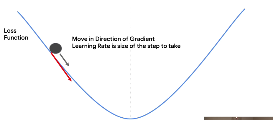
You're closer to the bottom. You still don't know how far it is, but you're closer. So you can repeat the process.

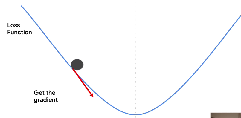
By differentiating again, you can get the gradient. And from the gradient, you can understand the direction towards the bottom. So you can move again in the direction of the gradient, and you'll end up here. Repeat the process again, and you could end up here. You're getting closer.

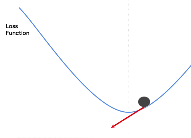
Another step and you'll be here, closer still. The next step could have us overshoot the bottom and end up here because of our step size. But that's OK, because when we differentiate from this spot, we'll have a new gradient pointing back towards the bottom. So we might end up here, overshooting again. And after a few steps, we could find ourselves oscillating over and back. But we're generally approaching the minimum.

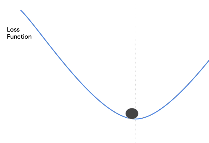
It's important to choose a good learning rate or we could oscillate forever. Or indeed, an advanced technique is to adjust the learning rate on the fly. It might be good to have it bigger when we're further up the curve and gradually reduce it step by step so that we can get to the bottom more quickly.

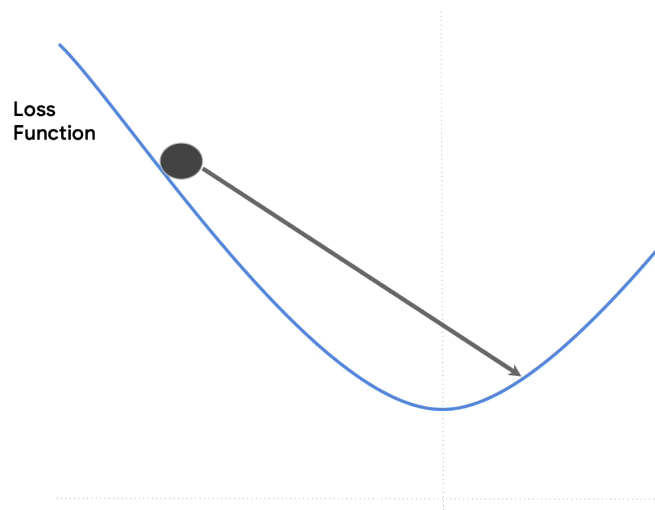
To illustrate, choosing the learning rate wisely is important. If it's too large, we could overshoot like this and then overshoot again on the way back like this and then overshoot again like this. We're never actually reaching the minimum.

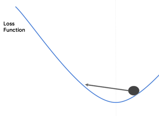
Or if the learning rate is too small, it might take a long timeto reach the minimum, a long, long, long time. Tiny increments will get you there. But as you can see, it's not the most efficient way.

Check out the code

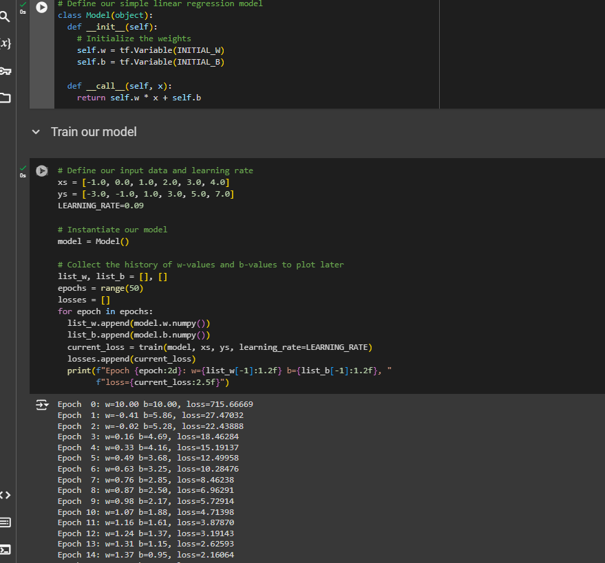
First Neural Network

Let's solve the problem with neura network

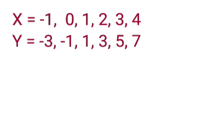
We have a bunch of x's and a bunch of y's. And we want to figure out the relationship between them. Earlier, we used the process of machine learning-- guessing, measuring, optimizing by hand, and we got the result y equals 2x minus 1. Let's now see how a neural network would do this.

Here is the code:

Let's break it down

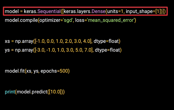
So I'll break it down line by line. This first line defines our model, and it's the simplest neural network that I could think of.

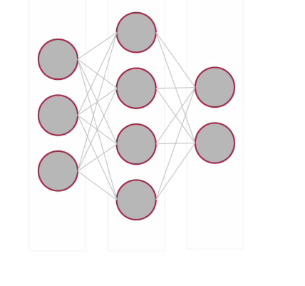
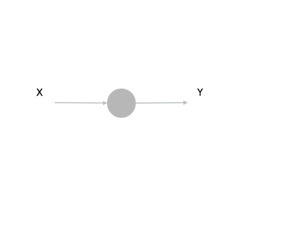
Each of these circles will be considered a neuron.

Each of these sets of neurons is called a layer.

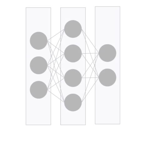
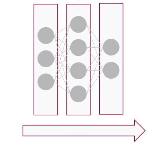
These layers are also in sequence. The first layer feeds the second which feeds the third.As a result, we'll use the term sequential to define this network. You might also have heard the term hidden layers when dealing with neural networks. The hidden layers are the middle ones that are neither input nor output.

So that middle one, you can see here, is a hidden layer.

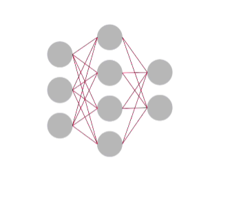
The neurons are all connected to each other, making a dense connection. And we'll use that term to define the name and the type of the layers.

So, let's break down the code

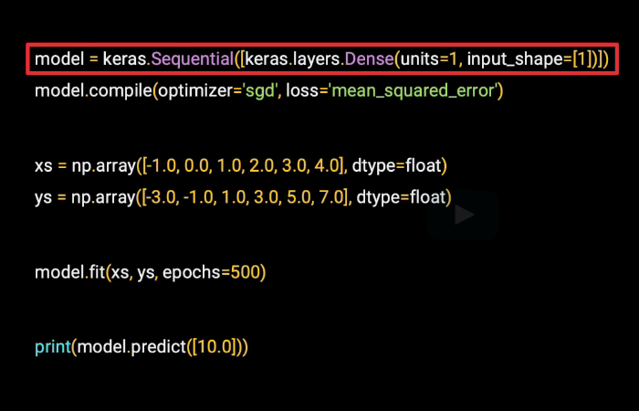
So now if we go back to our code, we can see the term sequential. We're defining a sequential neural network. Within the brackets, we would then list the layers in this neural network. We only have one entry, so we only have one layer. This layer is a dense, so that we know it's a densely connected network. The units parameter tells us how many neurons will be in the layer. And we can see that we only have one.

So this code defines the simplest possible neural network. There's one layer and it has one neuron.

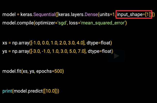
There's one other thing to call out when defining the first, and in this case the only, layer in a network, you have to tell at the input shape.

Now here our input shape has only one value. We're training a neural network on single x's to predict single y's. So again our input shape really couldn't be any simpler.

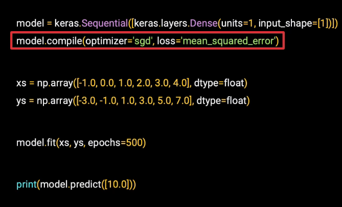
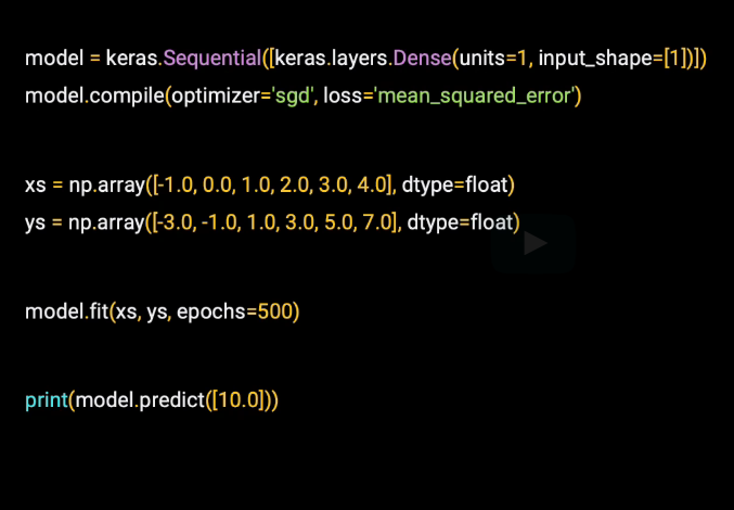
When we compile the model, we'll define the loss function and an optimizer. The loss function is mean squared error, as we used previously. But instead of calculating everything ourselves, we can just tell TensorFlow to use this last function for us. The optimizer is SGD, which stands for Stochastic Gradient Descent. And this will follow the process we saw in the previous video of using a gradient to descend down the loss curve to try and reach a minimum.

We're not doing any of the math or the calculus ourselves we'll just let TensorFlow do it for us.

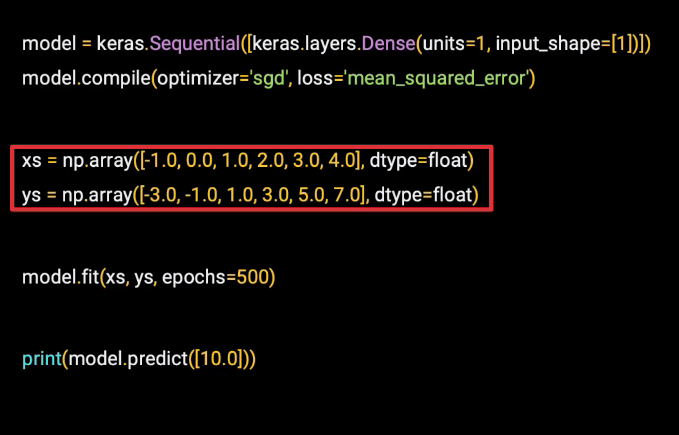
Now we specify the x's and the y's. TensorFlow expects these to be in a numpy array, and that's what that np stands for. And you can see that the array of y's has the corresponding y for a value in the x. So y equals minus 3 when x equals minus 1, y equals minus 1 when x equals 0, and so on.

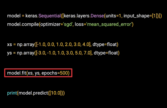
The process of figuring out this relationship or training is called fitting. So we do model.fit. We're fitting the x's to the y's. We'll do this for 500 epochs, where an epoch is each of the steps that we had discussed previously-- make a guess, measure the loss of the guess, optimize, and continue. So this line of code will do that 500 times. Then when we're done, we can use the model to predict the y for a given x.

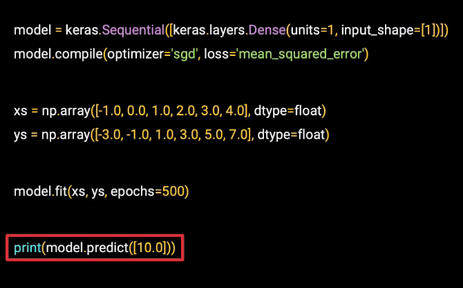
So if x is 10.0, what do you think y will be? Well, you can try it out for yourself now.

Check out the code

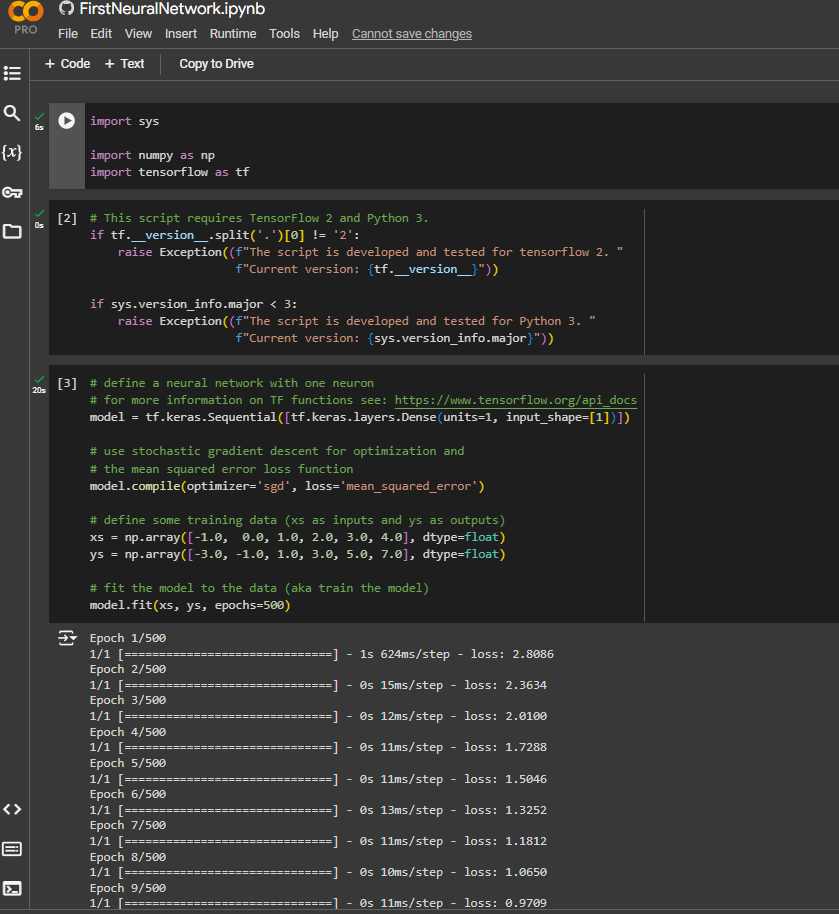
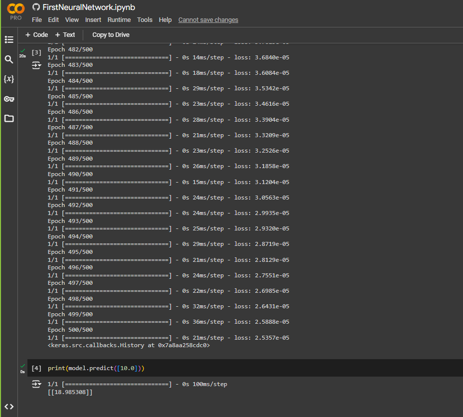
It did run for 500 times and you can see for value 10 as x, we get 18.98 as output.

Up to now you’ve been looking at matching X values to Y values when there’s a linear relationship between them. So, for example, you matched the X values in this set [-1, 0 , 1, 2, 3, 4] to the Y values in this set [-3, -1, 1, 3, 5, 7] by figuring out the equation Y=2X-1.

You then saw how a very simple neural network with a single neuron within it could be used for this.

This worked very well, because, in reality, what is referred to as a ‘neuron’ here is simply a function that has two learnable parameters, called a ‘weight’ and a ‘bias’, where, the output of the neuron will be:

Output = (Weight * Input) + Bias

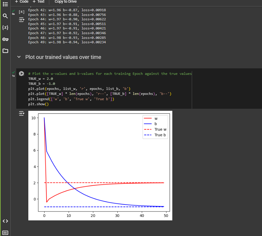
So, for learning the linear relationship between our Xs and Ys, this maps perfectly, where we want the weight to be learned as ‘2’, and the bias as ‘-1’. In the code you saw this happening.

When multiple neurons work together in layers, the learned weights and biases across these layers can then have the effect of letting the neural network learn more complex patterns.

In your first Neural Network you saw neurons that were densely connected to each other, so you saw the Dense layer type. As well as neurons like this, there are also additional layer types in TensorFlow that you’ll encounter. Here’s just a few of them:

• Convolutional layers contain filters that can be used to transform data. The values of these filters will be learned in the same way as the parameters in the Dense neuron you saw here. Thus, a network containing them can learn how to transform data effectively. This is especially useful in Computer Vision, which you’ll see later in this course. We’ll even use these convolutional layers that are typically used for vision models to do speech detection! Are you wondering how or why? Stay tuned!

• Recurrent layers learn about the relationships between pieces of data in a sequence. There are many types of recurrent layer, with a popular one called LSTM (Long, Short Term Memory), being particularly effective. Recurrent layers are useful for predicting sequence data (like the weather), or understanding text.

You’ll also encounter layer types that don’t learn parameters themselves, but which can affect the other layers. These include layers like Dropouts, which are used to reduce the density of connection between dense layers to make them more efficient, Pooling which can be used to reduce the amount of data flowing through the network to remove unnecessary information, and lambda lambda layers that allow you to execute arbitrary code.

Understanding Neurons