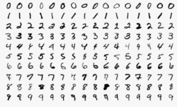
For the past few days I've been learning about Convolutional Networks and how they've transformed the field of Computer Vision and Deep Learning.

So, I decided to recreate the LeNet-5, the ALL TIME CLASSIC Convnet published by Yann LeCun in his paper titled Gradient-Based Learning Applied to Document Recognition in 1998.

And, as they say, old is gold. That's very much true for this Convnet, since, despite being older than me (I'm 21), it gave an accuracy of 99.8% on the MNIST training set!

In this article, you'll learn how to recreate this classic Convnet in Tensorflow. Feel free to comment down any questions that you have!

Code

First off, here are all the imports that you will need for this code.

These can be the dependencies that you may need to install if you're trying to run locally. Or you may use Google Colab and not worry about dependency issues at all.

import numpy as np # linear algebra
import pandas as pd # data processing, CSV file I/O (e.g. pd.read_csv)
import tensorflow as tf
import seaborn as sns
import matplotlib.pyplot as plt
import matplotlib.image as mpimg

I worked on the MNIST dataset that comes preloaded in the TensorFlow Dataset (TFDS). Store the dataset into two tuples of train and test data as shown below.

mnist = tf.keras.datasets.mnist
(x_train, y_train), (x_test, y_test) = mnist.load_data()

Now that you have your training and test data, it's time to carry out some EDA (Exploratory Data Analysis).

Firstly, let's check the dimensions of the dataset.

print("X train shape:", x_train.shape)
print("Y train shape:", y_train.shape)
print("X test shape:", x_test.shape)
print("Y test shape:", y_test.shape)

---------------------------Output-----------------------------
X train shape: (60000, 28, 28)
Y train shape: (60000,)
X test shape: (10000, 28, 28)
Y test shape: (10000,)

There are 60,000 examples available for training and 10,000 examples for testing in the MNIST dataset in TFDS.

Each example in the training (X) and test (X) dataset is a 28x28x1 image. Here's how you can view an image at any given index value.

index = 19
print(np.argmax(y_train[index]))
plt.imshow(x_train[index][:,:,:])

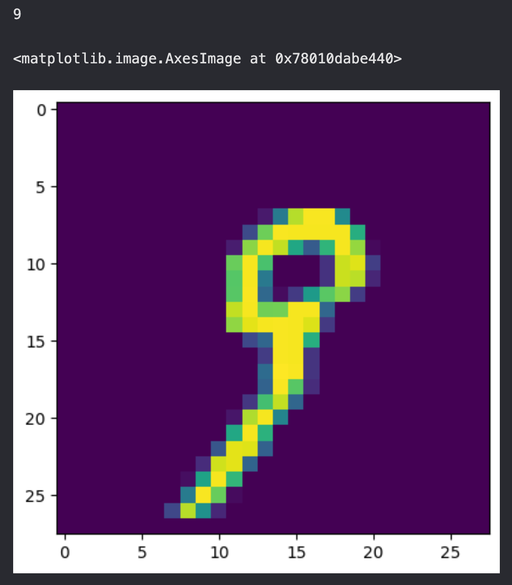
Since these are greyscale images, they only have one colour channel. However, the input dimensions do not explicitly represent the number of colour channels.

Hence, let's transform the train and test datasets to match tensorflow requirements for input data.

input_shape = (28,28,1)

x_train= x_train.reshape(x_train.shape[0], x_train.shape[1], x_train.shape[2], 1)
x_train= x_train / 255.0 #normalize the dataset
x_test = x_test.reshape(x_test.shape[0], x_test.shape[1], x_test.shape[2], 1)
x_test= x_test/255.0 #normalize the dataset

Here's how the x_train and x_test look after transformation:

print("X train shape:", x_train.shape)
print("X test shape:", x_test.shape)

---------------------------Output-----------------------------
X train shape: (60000, 28, 28, 1) 
X test shape: (10000, 28, 28, 1)

Now, the shape of the Xs explicitly include the number of channels as well!

Before building the model, there's one last thing to do, let's check the distribution of labels in y_train, to see if there isn't any single, or a group of labels that dominate the target values.

To check this, we plot a histogram of y_train.

sns.histplot(y_train)

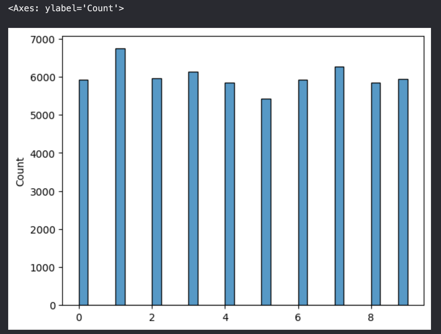
As you can see, almost all the numbers from 0 to 9 have similar number of examples corresponding to them, so we're good to go! Up next, let's build the LeNet-5!

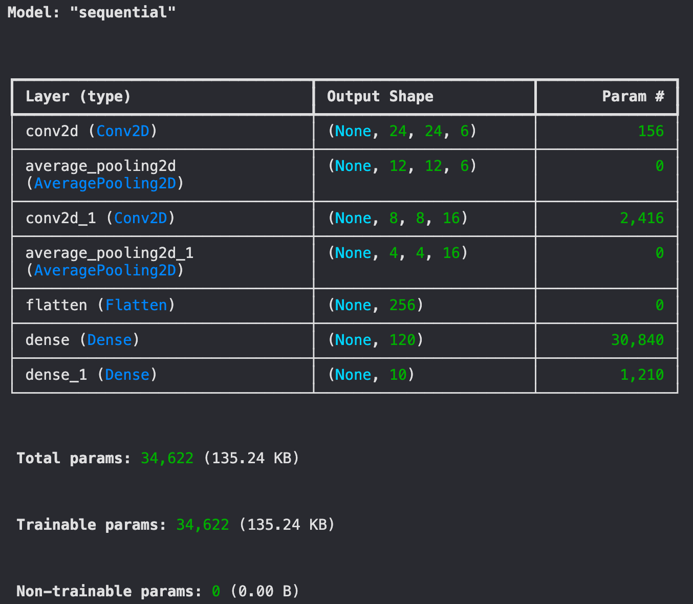
Since the dataset is composed of images of shape (28,28,1), the shapes of the intermediate outputs from the convolutional and pooling layers will be different than that defined in the orignal research paper.

However, since the layers that we apply are the same as in the research paper, the number of parameters will remain the same.

Let's build the model using the Sequential API of tensorflow.

model = tf.keras.models.Sequential([
    tf.keras.layers.Conv2D(6, (5,5), activation='tanh', input_shape=(28,28,1)),
    tf.keras.layers.AveragePooling2D(pool_size = 2, strides = 2),
    tf.keras.layers.Conv2D(16, (5,5), activation='tanh'),
    tf.keras.layers.AveragePooling2D(pool_size = 2, strides = 2),
    tf.keras.layers.Flatten(),
    tf.keras.layers.Dense(120, activation='tanh'),
    tf.keras.layers.Dense(10, activation='softmax')
])

##Learning: Sparse Categorical Entropy loss is used when the target variable isn't one hot encoded, else use categorical cross entropy loss
model.compile(optimizer="adam", loss='sparse_categorical_crossentropy', metrics=['accuracy'])

Here's the model summary.

model.summary()

Here, we use the Adam (Adaptive Moment Estimation) optimizer to update the parameters after every forward pass. And, we use the Sparse Categorical Cross Entropy loss to measure the performance of the model.

What are we waiting for? Let's train the model!

history = model.fit(x_train, y_train,
                    batch_size=10,
                    epochs=20,
                    validation_split=0.1)

We split the training dataset into 90% training and 10% validation set. This is done to effectively measure the accuracy of the model before we test it on the testing dataset. This is what the "validation_split=0.1" does.

And, here are the results!

---------------------------Output-----------------------------
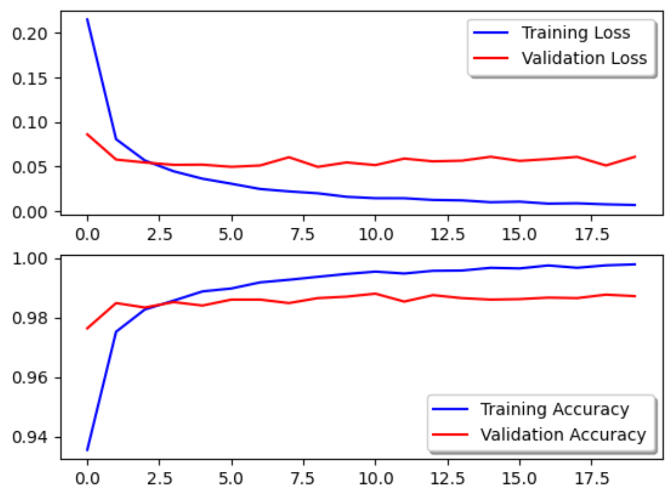
Training Accuracy: 99.81%
Training Loss: 0.006
Validation Accuracy: 98.72%
Validation Loss: 0.0609

Look at the progression of the accuracy and the loss through the number of epochs.

fig, ax = plt.subplots(2,1)
ax[0].plot(history.history['loss'], color='b', label="Training Loss")
ax[0].plot(history.history['val_loss'], color='r', label="Validation Loss")
legend = ax[0].legend(loc='best', shadow=True)

ax[1].plot(history.history['accuracy'], color='b', label="Training Accuracy")
ax[1].plot(history.history['val_accuracy'], color='r',label="Validation Accuracy")
legend = ax[1].legend(loc='best', shadow=True)

Finally, let's evaluate how the model does on the test set.

test_loss, test_acc = model.evaluate(x_test, y_test)

---------------------------Output-----------------------------
Test Accuracy: 98.37
Test Loss: 0.0599

And that's a wrap! That's how you recreate the LeNet-5 and achieve such high accuracy on the MNIST dataset.

In this article, I demonstrated how you recreate the classic Convnet LeNet-5 that recognizes handwriting, and works exceptionally well on the MNIST dataset.

Subscribe to my newsletter for more such articles!