Unboxing Neural Networks (A Quick Summary)

Have you ever wondered how neural networks magically "learn"? I have been coding for a few years and whenever I wanted my computer to do something, I'd have to explicitly instruct it to do it. The concept that computers could learn to do tasks fascinated me a lot. Although I had trained a few neural networks (mostly to quench my curiosity about their inner workings), I could not figure out how a neural network could learn. So I decided to code my own neural network from scratch. Here's what I've learnt.

The network itself is a very complex math function. It takes in features of the data as parameters and produces an output. During training the network tries to learn patterns in the data.

Let's consider an example neural network.

It takes in an input X and produces an output a3. L1, L2 and L3 are the different layers of this neural network, each with a single neuron to keep the network simple.

How does this network "learn"?

Well, the learning process can be divided into 3 steps:

1. Forward Propagation

2. Calculating Loss

3. Backward Propagation

Forward Propagation

The data flows from left to right. All the weights (w1, w2 and w3) and biases (b1, b2 and b3) are initialised randomly. For the first layer, the input X is multiplied by its corresponding weight which is w1 and the result is summed with b1. So

\begin{equation} a_1 = X \cdot w_1 + b_1 \end{equation}

Similarly,

\begin{equation} a_2 = a_1 \cdot w_2 + b_2 \end{equation}

\begin{equation} a_3 = a_2 \cdot w_3 + b_3 \end{equation}

Now, a3 is our predicted value.

Calculating Loss

Let's assume that the true value is t. If we use a simple mean squared error loss function, the loss l is

\begin{equation} l = (a_3 - t)^2 \end{equation}

This value represents how much our output deviates from the true/actual value. Our objective is to minimise this deviation so that our predictions are close to the true value. How can we minimise the loss?

Backward Propagation

Another glance at our neural network will reveal that there are a few variables in our neural network. These are - w1, b1, w2, b2, w3 and b3 (a1, a2 and a3 are a result of some operations on these variables). By tweaking these variables we can tune our model to minimise the loss value y. But how do we figure out how much each variable should be changed? And more importantly, should we increase or decrease each variable's value?

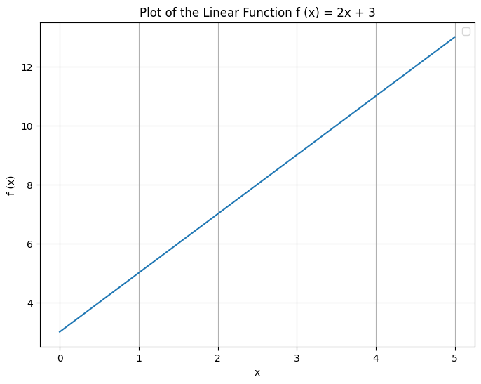
The answer lies in calculus! Let's consider a function \(f(x) = 2x + 3\)

If we compare it to the equation \(y = mx + b\), we find the slope to be 2. Another way to calculate the slope is to find the rate of change/derivative of f(x). Also,

\begin{equation} \frac{df(x)}{dx} = 2 \end{equation}

This tells us how much the input x to the function f(x) affects the output (magnitude of change). It also gives the direction of change of the output with respect to the input. In simple terms, it tells us if the input and output are positively or negatively correlated (direction of change). Also, note that there exists a value of x (-1.5 in this case) for which the function's output is 0.

Note: The gradient gives the direction and magnitude of the steepest ascent of the function. We move in the opposite direction of the gradient to reduce the output, hence it is also called gradient descent.

Now if we consider our neural network as a giant function, or rather a chain of functions, we will find that

\begin{equation} l = f(g(h(i(X)))) \end{equation}

where

\begin{equation} l = f(a_3, t) \end{equation}

\begin{equation} a_3 = g(a_2, w_3, b_3) \end{equation}

\begin{equation} a_2 = h(a_1, w_2, b_2) \end{equation}

\begin{equation} a_1 = i(X, w_1, b_1) \end{equation}

It is difficult to imagine this multivariate function graphically but we want some configuration of w1, b1, w2, b2, w3 and b3 for which the loss is minimum. Also, if we nudge each of these weights and biases individually in the opposite direction of their gradients we will move down along the graph.

The next step would be to calculate the partial derivatives of loss function with respect to each variable. Partial derivatives represent the change in a multivariate function with respect to each input variable of the function. The loss function is a chain of functions, so partial derivatives will be

\begin{equation} \frac{dl}{dw_3} = \frac{dl}{da_3} \cdot \frac{da_3}{dw_3} \end{equation}

dl/da3 represents how much the loss changes when a3 changes and in what direction while da3/dw3 represents how much da3 changes when dw3 is nudged.

Similarly,

\begin{equation} \frac{dl}{db_3} = \frac{dl}{da_3} \cdot \frac{da_3}{db_3} \end{equation}

\begin{equation} \frac{dl}{dw_2} = \frac{dl}{da_3} \cdot \frac{da_3}{da_2} \cdot \frac{da_2}{dw_2} \end{equation}

\begin{equation} \frac{dl}{db_2} = \frac{dl}{da_3} \cdot \frac{da_3}{da_2} \cdot \frac{da_2}{db_2} \end{equation}

\begin{equation} \frac{dl}{dw_1} = \frac{dl}{da_3} \cdot \frac{da_3}{da_2} \cdot \frac{da_2}{da_1} \cdot \frac{da_1}{dw_1} \end{equation}

\begin{equation} \frac{dl}{db_1} = \frac{dl}{da_3} \cdot \frac{da_3}{da_2} \cdot \frac{da_2}{da_1} \cdot \frac{da_1}{db_1} \end{equation}

Now that we have all the derivatives, we can update the weights and biases. One way to do this is stochastic gradient descent. In this, we subtract the product of gradients and a pre-defined learning rate from the current values of weights and biases.

Training the Neural Network

The network sees each piece of data and goes in cycles of the learning process (i.e. forward propagation, calculating loss and finally backward propagation) to update the weights and biases. The hopes from this layered structure is that it captures the nuances/ patterns in the data and updates weights and biases in such a way that it becomes generalised and whenever a new piece of data is passed on to it, it can gives a suitable output.

Need for Activation Functions

You might have realised that the network is simply a linear function of the form \( y = mx + b \) in a higher dimension. It would fail to recognise patterns in the data where the relationship between different inputs is non-linear. How do we introduce a non-linearity in our neural network function?

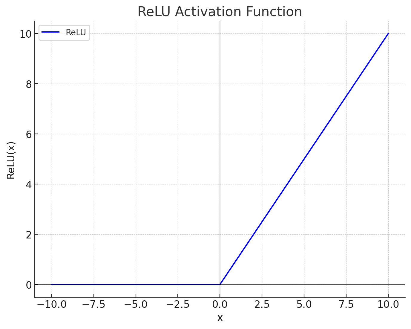
A simple way to do this is by using activation functions. A simple and widely used activation function is Rectified Linear Unit (ReLU). It is defined as

\begin{equation} \text{ReLU}(x) = \max(0, x) \end{equation}

The output of each neuron in a layer is forwarded through this function and the next layer is connected to the output of the ReLU layer. Introducing this simple non-linearity can capture complex patterns in the data provided that the neural network has enough layers and neurons per layer.