How to Create a Keras-Style Neural Network from Scratch

Deep learning, leveraging multi-layered neural networks, has gained popularity due to enhanced computational power and large datasets. It excels in image and speech recognition, NLP, autonomous driving, and healthcare diagnostics, transforming industries by automating complex tasks and enabling high-accuracy data analysis and decision-making.

Creating a neural network from scratch can significantly deepen your understanding of how modern deep learning frameworks like Keras operate. This guide will walk you through the theoretical aspects of building a neural network, covering layers, activation functions, loss functions, and optimization techniques.

Neurons

Neurons in neural networks are computational units that mimic biological neurons.

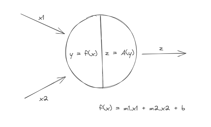
Each neuron calculates own weight (m1, m2) for each input (x1, x2). They receive input, apply a weighted sum, add a bias, and pass the result (y) through an activation function. Activation functions tell whether a neuron is "on" / "off".

This is a single neuron, when organized in layers, they create a neural network.

Chain rule

Let's look at this simple example

The steps which take place are as follows

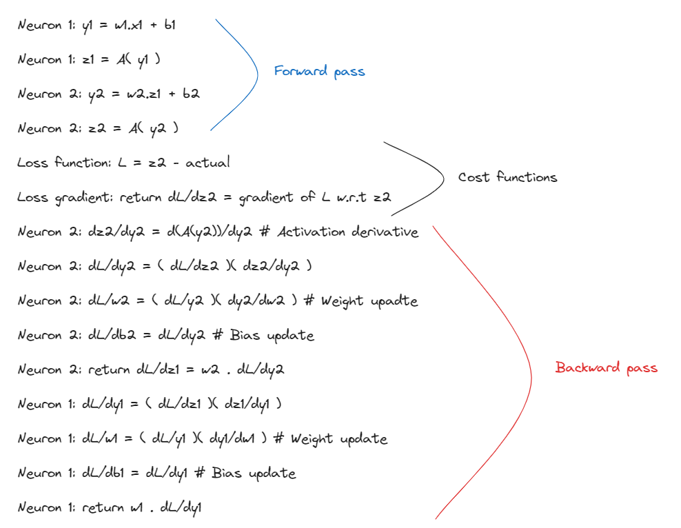
However this computation is clubbed together to form a chain

Thus the final output or the prediction is just a chained operation of the selected output and activation functions.

Dense Neural Network

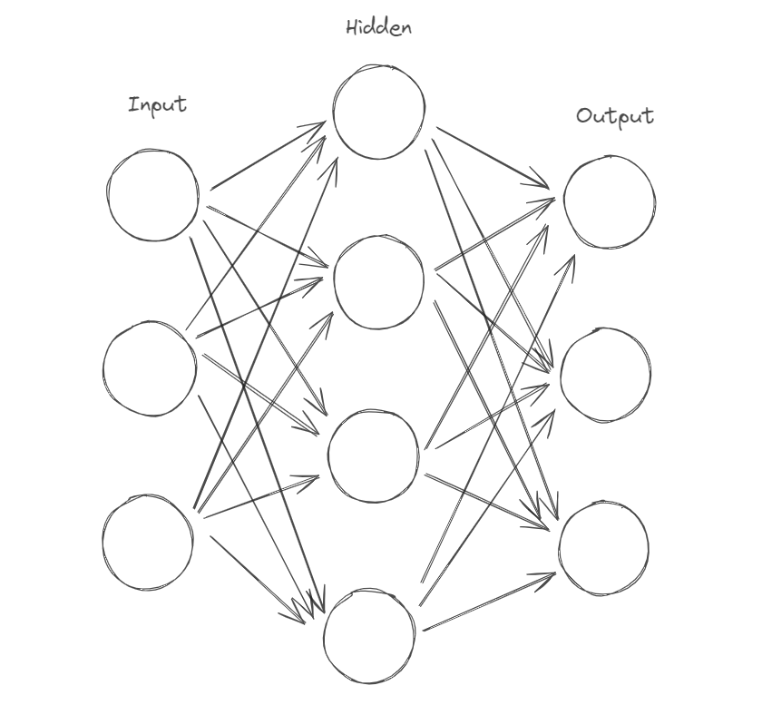
This is called a "Dense" layer where every neuron is connected to every neuron of the succeeding layer. Some famous libraries used to create a neural network are Keras, Tensorflow, Pytorch, etc.

Previously we saw that neuron computes y = w.x + c. But here we have 4 neurons. so the output of the layer will not be a single value but a row [ y1, y2, y3, y4 ]. And if we have multiple input samples ( input rows ), each y will itself be a row of values for each sample. Therefore, the output of a layer will be a matrix.

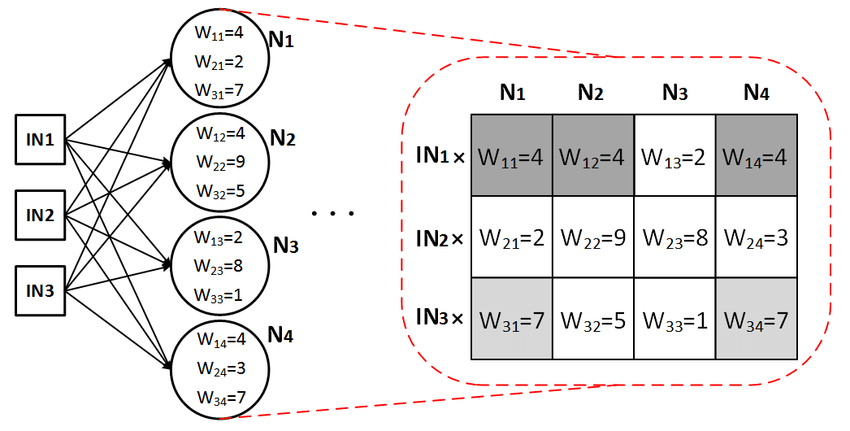
Notice how a matrix represents an entire layer. In the picture, the matrix holds values for different neurons in different columns. You can also use the transpose to get each neuron in different rows instead of columns; either way works.

On studying a simple 1x1 neural network, we saw with the chain rule how many computations take place. However, this structure, even though it looks complex, is not hard to implement. We only need to create and update two matrices (for two layers) once in each epoch. Let's create this from scratch using just numpy.

Building from Scratch

import numpy as np
import pandas as pd # only for data saving/extracting purposes

We will use the principles of Object Oriented Programming using Python to create classes and objects for layers and neural networks.

Layer

class Layer:
    def __init__(self, output_size, input_size, activation="none"):
        self.weights = np.random.rand(output_size, input_size)
        self.bias = np.random.rand(output_size, 1)
        self.__activation = Activation(activation)

    def activate(self, X):
        return self.__activation.activate(X)

    def activation_derivative(self):
        return self.__activation.activate_derivative(self.output)

You can see that I have defined a Layer class which will be inherited by sub classes to create "Dense" or "Sparse" layers. Since each layer has its activation function, we need to implement activation class for dynamic activations.

Activation function

class Activation:
    def __init__(self, func):
        self.__func = func

    def activate(self, X):
        if self.__func == "relu":
            return np.maximum(0, X)
        elif self.__func == "softmax":
            exp_values = np.exp(X - np.max(X, axis=1, keepdims=True))
            return exp_values / np.sum(exp_values, axis=1, keepdims=True)
        else:
            return X

    # calculates gradient for activation
    def activate_derivative(self, X):
        if self.__func == "relu":
            return np.where(X > 0, 1, 0)
        elif self.__func == "softmax":
            return X
        else:  # no activation
            return np.ones_like(X)

Now let's create a dense layer

Dense Layer

class Dense(Layer):
    def __init__(self,output_size, input_size, activation="none"):
        Layer.__init__(self, output_size, input_size, activation)

    def forward_pass(self, data):
        self.input = np.array(data)
        y = np.dot(self.weights, self.input) + self.bias
        self.output = self.activate(y) # -- activation
        # self.output = y # -- no activation
        return self.output

    def backward_pass(self, loss_gradient, learning_rate):
        activation_gradient = self.activation_derivative()
        # dl/da -- gradient for activation
        output_gradient = loss_gradient * activation_gradient
        # dl/dy -- gradient for output
        weights_gradient = np.dot(output_gradient, self.input.T)
        # dl/dw -- gradient for weights
        self.weights -= learning_rate * weights_gradient
        self.bias -= learning_rate * np.sum(output_gradient, axis=1, keepdims=True)

        input_gradient = np.dot(self.weights.T, output_gradient)
        # transforming gradient for next layer

        return input_gradient

Sequential Network

class Sequential:
    def __init__(self):
        self.__layers = []

    def add(self, layer):
        self.__layers.append(layer)

    def forward_pass(self, data):
        output = data
        for layer in self.__layers:
            output = layer.forward_pass(output)
        return output

    def backward_pass(self, loss_gradient, learning_rate):
        for layer in reversed(self.__layers):
            loss_gradient = layer.backward_pass(loss_gradient, learning_rate)

    def compile_(self, loss):
        self.__loss = loss

    def fit(self, X, Y, epochs, learning_rate):
        X = np.array(X)
        Y = np.array(Y)
        for epoch in range(1,epochs+1):
            output = self.forward_pass(X)
            loss_gradient = self.__loss.gradient(output, Y)
            self.backward_pass(loss_gradient, learning_rate)
            loss_value = self.__loss.calculate(output, Y)
            #print at every 100th epoch
            if epoch % 100 == 0:
                print(f"Epoch {epoch}/{epochs}, Loss: {loss_value}")

    def predict(self, X):
        X = np.array(X)
        pred = self.forward_pass(X.T)
        res = np.mean(pred, axis=0)
        return [round(i) for i in res]

    # only for simplicity
    def coef(self):
        return self.__layers[-1].weights, self.__layers[-1].bias

We also require a "Loss" class for calculating cost and gradient.

Loss

class Loss:
    def calculate(self, output, y):
        raise NotImplementedError

    def gradient(self, output, y):
        raise NotImplementedError

This is a general class which can be inherited by different sub class like MSE, CrossEntropy, etc.

class MSE(Loss):
    def calculate(self, output, Y):
        n_samples = output.shape[1]
        loss = np.mean(np.mean((output - Y)**2 / 2, axis=1))
        return loss

    def gradient(self, output, Y):
        n_samples = output.shape[1]
        loss_gradient = (output - Y)/n_samples
        return loss_gradient

Data

def generate_random_samples(n_samples, a, b):
    # Generating random values for the first three columns
    return np.random.randint(a, b, size=(n_samples, 3))

random_samples = generate_random_samples(10000, 0, 100)
data = pd.DataFrame(random_samples, columns=['x','y','z'])
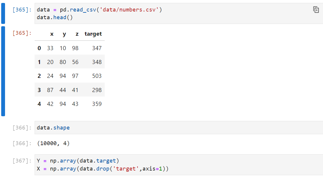
data['target'] = data['x'] + 2 * data['y'] + 3 * data['z']

# generated 10,000 rows of data where the target is calculated as:
# target = x + 2y + 3z

# you can save this to a file to avoid recalculation
data.to_csv('data/numbers.csv', index = False)

Train Test

Y = np.array(data.target)
X = np.array(data.drop('target',axis=1))

# for simplicity
X_train, X_test, Y_train, Y_test = X[:9000], X[9000:], Y[:9000], Y[9000:]

Model

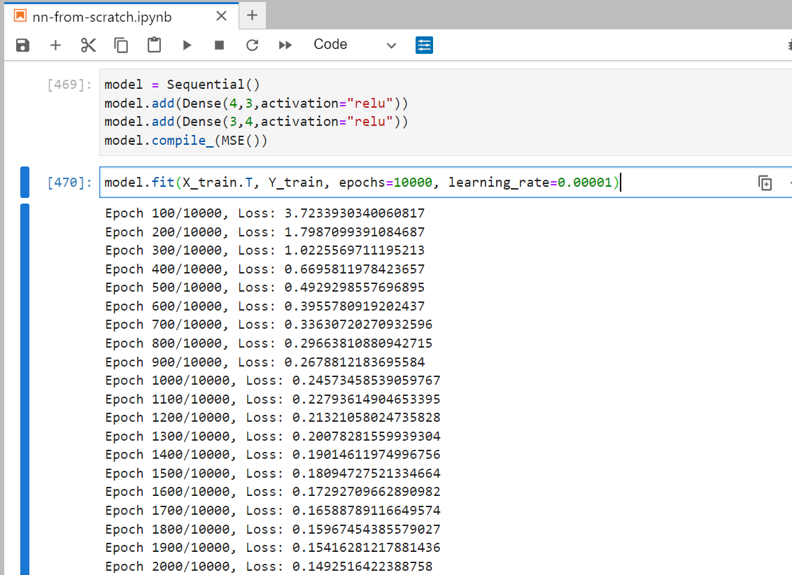
I have added two dense layers with 4 and 3 neurons respectively.

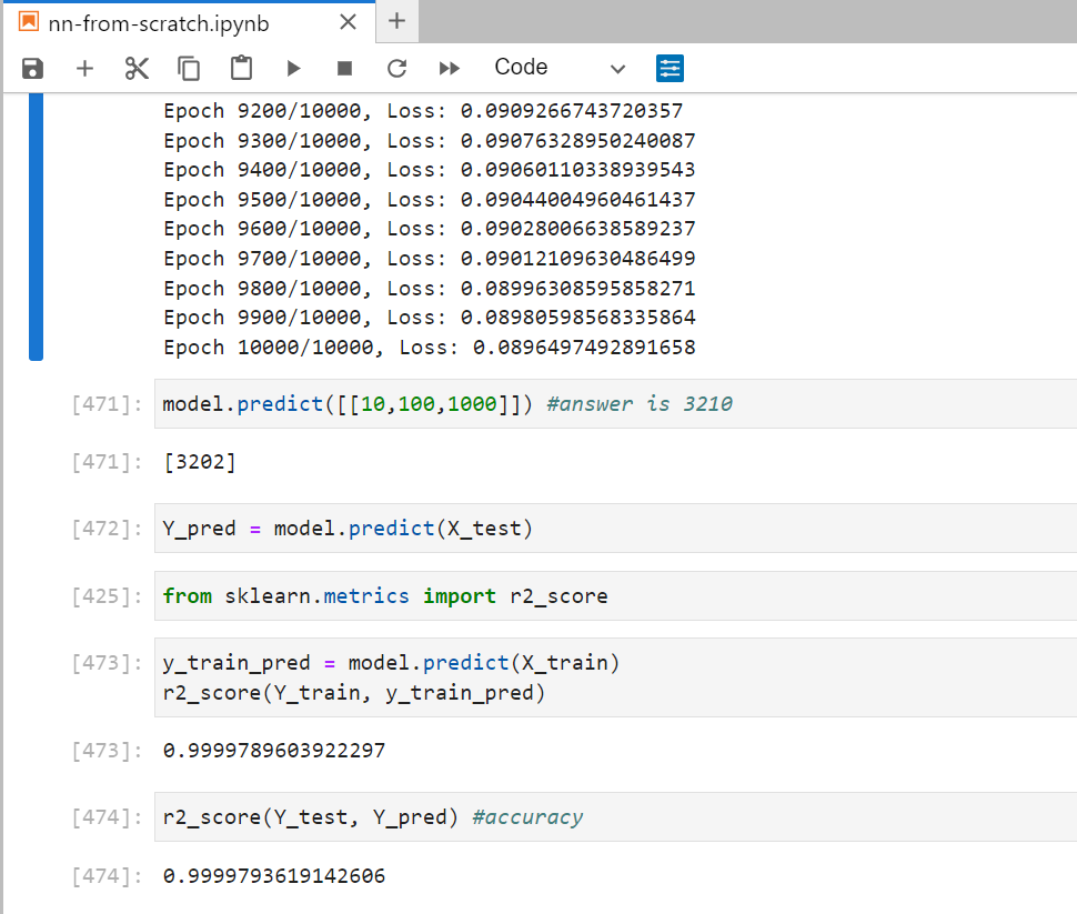
Super Easy!

More models

Let's create a simple 1 layer model comprising 3 neurons and see if it correctly adjusts weights and bias.

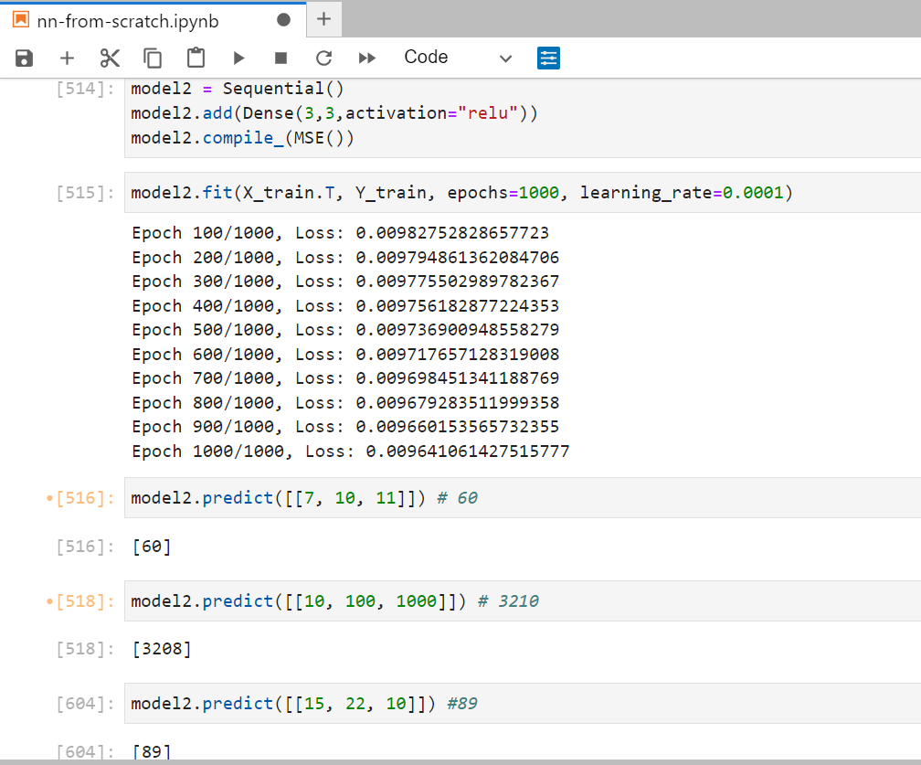
Model 2 needs fewer epochs and a higher learning rate because it is less complex than the previous one. You can try creating your own model based on your understanding and experiment with the parameters to find the optimal values. In the end, it's all about "Trial and Error".

Coefficients

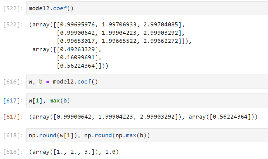
Notice that the three neurons in the output layer have weights close to 1, 2, and 3, which are our actual weights. The biases are 0.49, 0.16, and 0.56, while our bias is 1.

In a more complex neural network, the coefficients are not calculated the same way. This is because multiple layers contribute to the output, so the weights are cumulative.

Activation significance

We know that our maximum bias is 0.56, which is the closest to the actual value among the three. Therefore, after backpropagation, this specific neuron and the preceding neurons that contribute to this outcome will become more active. This means the value after activation will get higher or "brighter". For neurons that are farther from the actual value, they will get "dimmer", meaning their output after activation will be even lower.

A high activation means that the neuron is more closer to the truth. Look at this example.

This is a complex dense neural network with 3 hidden layers. For each neuron, the whiter it gets, the more "active" it is, and therefore, the more "relevant" it is. The leftmost neurons are the input features. The black ones indicate that these features are the least important or "irrelevant," while the white ones are the most important features.

Validate

Let's see if our model is generalized and works on higher numerical values

from sklearn.metrics import r2_score

# 100 samples between 5000 and 10000
test_samples = generate_random_samples(100, 5000, 10000)
m = np.array([1, 2, 3])
y_high_test = np.sum(test_samples * m, axis=1)

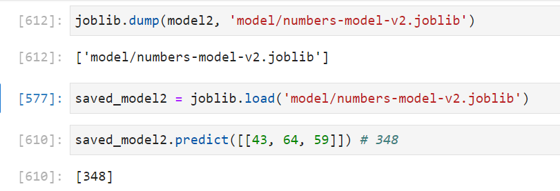
Save the model

Github

The entire code is available on my Github repository. Follow the link:

Hellcaster99/nn-from-scratch

Conclusion

We successfully created a Keras-style neural network for regression by understanding the chain rule and using OOP with Numpy and Python. This helped us gain a deeper understanding of how deep neural networks compute outputs.

Thanks for reading it through! I hope you liked it. Feel free to like and comment any doubt or suggestion regarding any topic. You can also reach out to me on my social in my bio. I am open to discussion :)