Probability & Statistics for Machine Learning & Data Science

Lesson 1 - Introduction to Probability

Probability is the likelihood of an event occurring. Let's get into it.

Let's say, In a school there are 10 kids where 3 kids plays football and 7 kids don't play football. What will be the probability of picking a random kid who plays soccer? We will use P(football) to denote the probability.

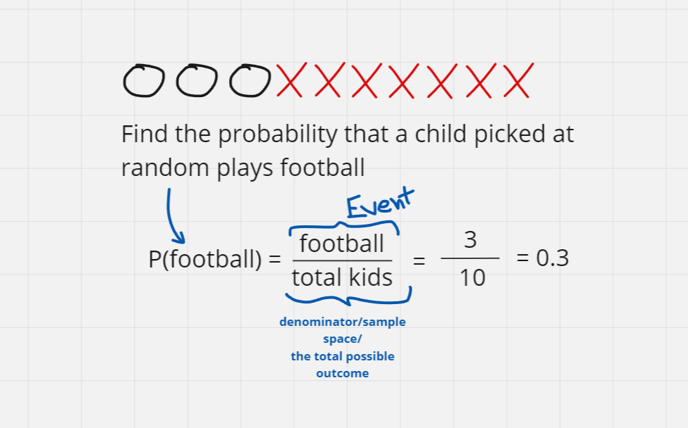
To find how many kids plays football. we need to know the number of total kids. 3 kids plays football, that's the size of the event. The sample space's size is 10. then we divide event by sample space.

Coin Example

Flipping a coin :

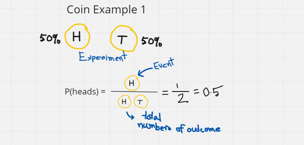
When we flip a coin, it can land on heads or tails. We don't know which one is likely to occur. As, the result is uncertain we are going to call it an experiment. In probability, an experiment is any kind of process that produces an uncertain result. In this coin flipping test, the experiment is throwing the coin. Here, both of the outcomes (H/T) has 50% possibility to occur.

Now, what will be the probability if we flip two coins and both of them lands on heads?

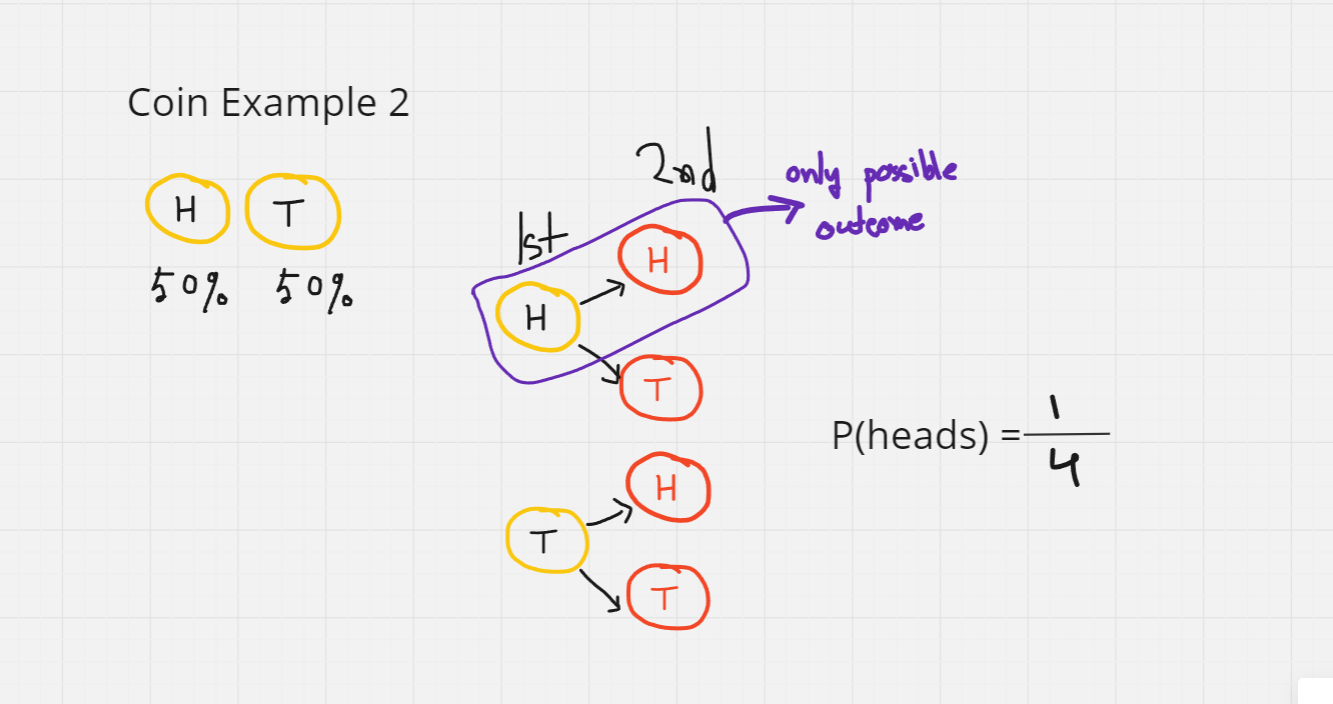
1st coin can lands on H/T. Following the 1st outcome, 2nd one can land on heads or tails. So, the total possible outcomes are HH,HT,TH,TT. The only possible outcome where it lands both on heads is HH.

Now, what if we flip three coins?

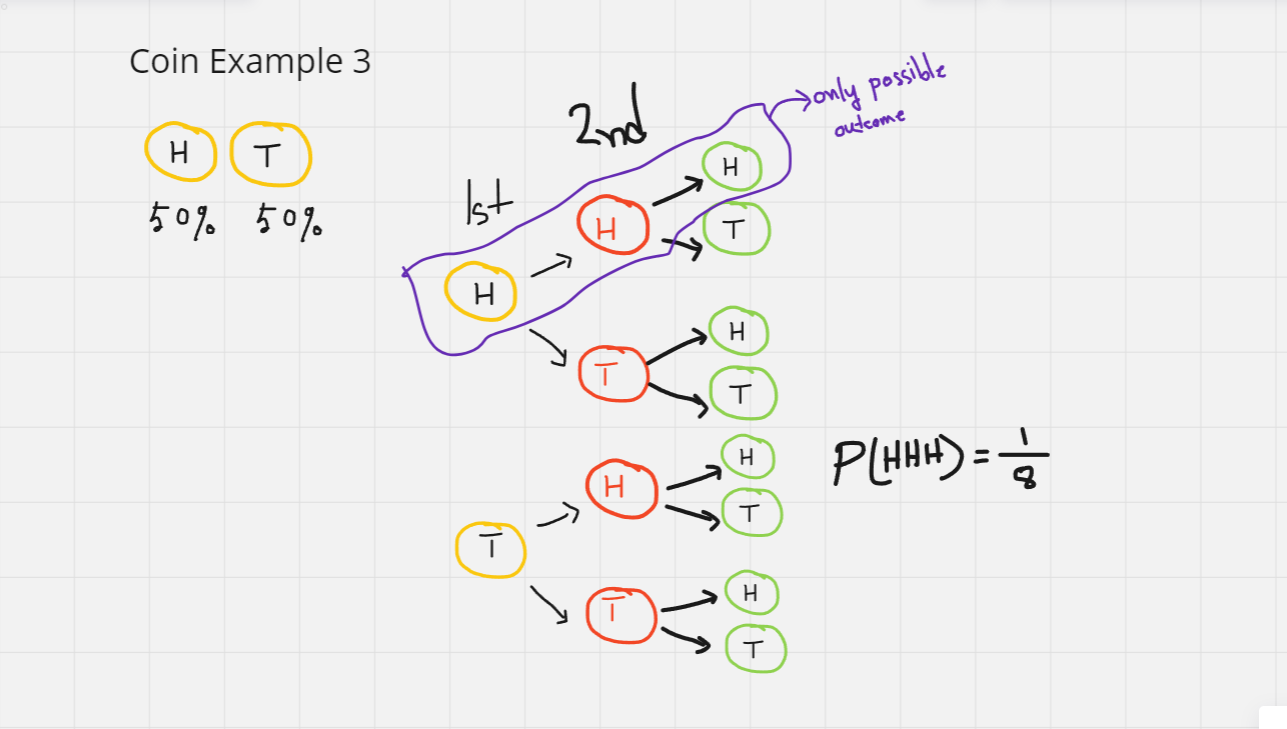
Same as before, 1st coin can lands on H/T. Following the 1st outcome, 2nd one can land on heads or tails. Thus, 3rd outcome can be also land in heads or tails. There are 8 possible outcomes - HHH,HHT,HTH,HTT,THH,THT,TTH,TTT. What will be the probability of landing heads thrice? P(HHH) will be 1/8.

Dice Example

Rolling a six sided dice:

If you roll a 6 sided dice, what is the probability of getting a 6? As there are six sides, so the possible outcome will be six and only one side is embedded with six dots so the event is one, Hence, the possibility of getting a six is 1/6.

Rolling two six sided dice:

If you roll two six sided dice, what is the probability of getting 6,6? We have six possibilities for each dice. So the total possible outcome or, the sample space is 36. From landing 1 1, 1 2, 1 3, 1 4, ....5 4, 5 5 ......6 4, 6 5, 6 6 - we get 36 in total. "6 6" is the only possible outcome, and the size is one. So, chance of getting two sixes is 1/36

Complement of Probability

Complement of probability is opposite of possibility. It means, the measurements of an even most likely to NOT OCCUR.

Let's get back to the first example of the blog and calculate the complement of probability.

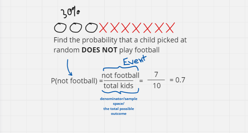
As usual, we count how many kids do not play football. In this case, 7 kids do not play football, so 7 is the event here.

Now, the interesting and important fact is, if we add P(not football) + P(football) -> 0.7+0.3 = 1. This always happens and we can rewrite this as P(not football) = 1 - P(football).

P(not occurring) = 1 - P(occurring) or,

P(A') = 1 - P(A) This is the Complement rule

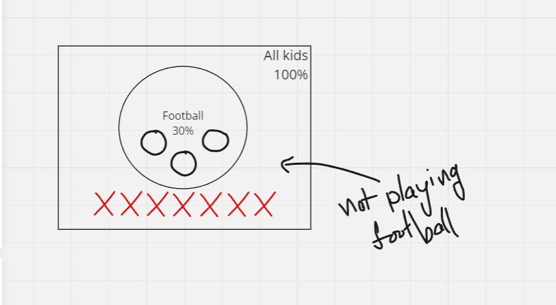
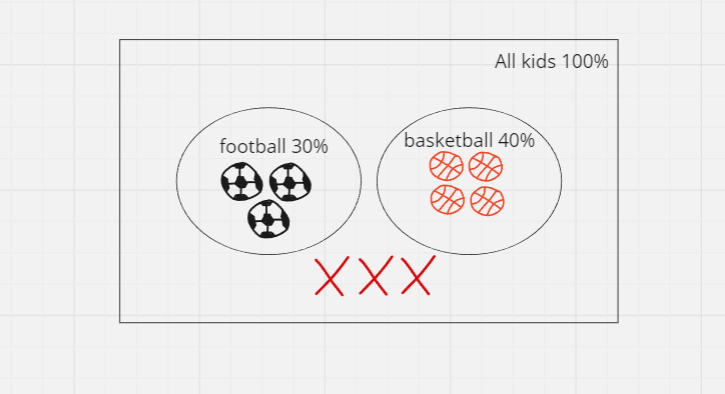
Venn diagram: Event of not playing football is everywhere outside of the circle, which is 70% (Circle is 30%).

Now, if we recall the coin experiment, what's the probability of not getting HHH? Using the complement rule, P(HHH') = 1 -P(HHH) => 1 - 1/8, and the result is 7/8.

What is the probability of obtaining anything other then six in a six sided rolling dice? P(not 6) = 1 - P(6) => 1-1/6 => 5/6

Sum of Probabilities (Disjoint Events)

Definition: Disjoint events (also known as mutually exclusive events) are two or more events that cannot occur simultaneously. If one event occurs, the other cannot.

Sum of probabilities are quite simple. Imagine, getting 1 or 2 in the roll of a dice. If we know the probability of getting 1 and 2, then we just need to add them up. But there's an edge case, it does not always work. We need to figure out if the events are disjoint or not for this.

Let's see the school example with more information.

At a school, there are 10 kids and they can play only one sport, either football or basketball. P(F) = 0.3 and P(B) = 0.4. What is the probability of a kid plays basketball or football?

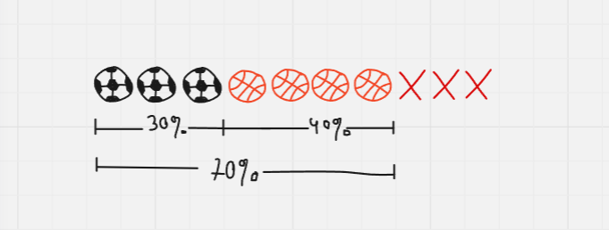
P(football or basketball) = football or basketball / total => (0.3+0.4)/10. Did you notice we just added the possibilities?

We will write this as the union of basketball and football. The formula is written as A∪B = P(A) + P(B)

Venn diagram:

Dice example - 1: In a 6-side dice, what is the probability of getting an even number or a 5? Ans : 2/3

There are two events here - getting evens that is 3/6 and getting 5, that is 1/6. If we add them, we get 2/3. P(even or 5) = P(even num) + P(50 = 2/3

Dice example - 2 : What is the probability of getting a sum of 7 or sum of 10?

Event A = Sum of 7; Event B = Sum of 10

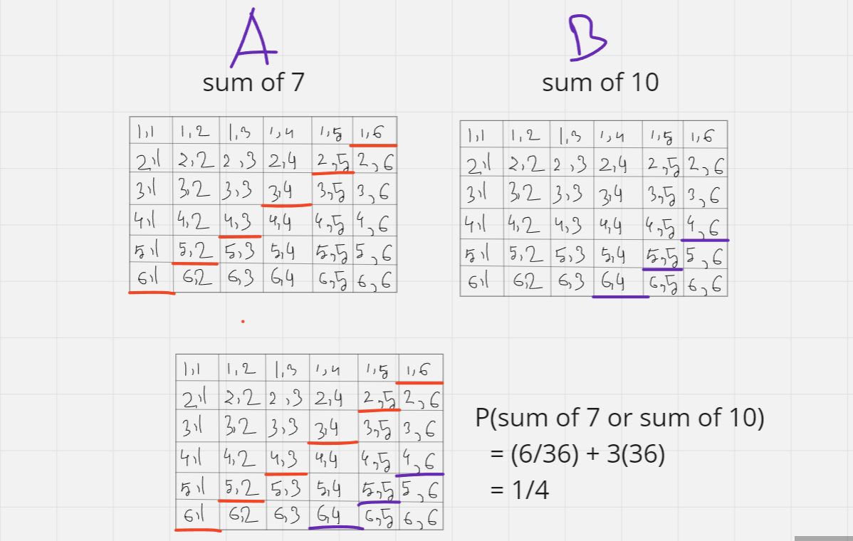
Orange marks the ones that turn 7 after adding. Purple marks get 10 after adding. If we union both of them, the probability of getting a sum of 7 or 10 is 1/4.

Find the P(difference of 2 or difference of 1). Remember, it can go both ways. The answer will be 18/36.

Sum of Probabilities (Joint Events)

What happens if the events are not joint? Do we still add them? No, that's not possible. In real world occurrences, events are mostly joint events.

To solve, again, back with the school situation - At a school there are 10 kids, they can play as many sports as they want. Given, P(S) is 0.6 and P(B) is 0.5. What is the probability of a kid playing soccer or basketball?

Is it P(S) + P(B)? But, it results in 11. Isn't it abnormal? So, We cannot tell with the information given, right? Well, let's get some more information now. Let's approach differently,

6 kids plays soccer |S| = 6, 5 kids plays basketball |B| = 5 and 3 kids plays both of them |S∩B| = 3. How many kids plays soccer or basketball? The answer is 8 because 5 + 6 - 3 = 8

Explanation : 5 plays basketball, 6 plays soccer, and 3 plays both so that's 8 because 2 of the kids don't play any sports.

The formula is, for any two events A and B: P(A∪B)=P(A)+P(B)−P(A∩B). This is also known as the inclusion-exclusion principle.

Now, back with the previous question - Given, P(S) is 0.6 and P(B) is 0.5 and P(S∩B) = 0.3; What is the probability of a kid playing soccer or basketball?

HINT : P(A∪B)=P(A)+P(B)−P(A∩B)

Venn diagram :

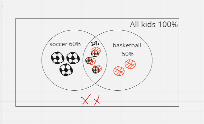
The diagram shows, the events are not mutually exclusive.

Dice Example 1 : What is the probability of achieving a sum of 7 or a difference of 1?

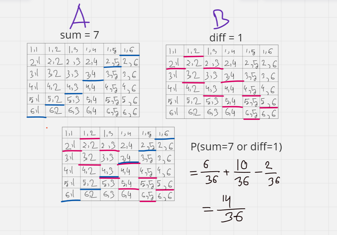
We have double counter (4,3) and (3,4). So we gotta subtract them in order to remove errors. So that is P(sum of 7) + P(diff of 1) - P(sum 7 ∩ diff 1) = 14/36

Independence

When an event occurs but does not influence or affect the possibility of occurring any other event is basically called Independence.

For example : Drawing Cards with Replacement

Scenario: Drawing a card from a deck, replacing it, and then drawing another card.

Events:

• Event A: Drawing an Ace on the first draw.

• Event B: Drawing a King on the second draw.

Explanation: Since the card is put back after the first draw, the deck stays the same for the second draw. This means the result of the first draw does not affect the result of the second draw, making events A and B independent.

Another example : Student Test Scores

Scenario: Two students taking the same test independently.

Events:

• Event A: Student 1 scores above 90%.

• Event B: Student 2 scores above 90%.

Explanation: Assuming the students do not collaborate and the tests are graded independently, the score of Student 1 does not affect the score of Student 2. Hence, events A and B are independent.

One more Example : Flipping Two Coins

Scenario: Flipping two coins simultaneously.

Events:

• Event A: The first coin lands on heads.

• Event B: The second coin lands on tails.

Explanation: The outcome of the first coin flip (heads or tails) does not affect the outcome of the second coin flip. Thus, events AAA and BBB are independent.

But, if I play chess, then my 12th move will affect the 13th move. Or, if it rains, the picnic gets canceled. These kinds of events influence the possibility of other events occurring. Hence, these types of events are not independent.

Understanding independency is very important in machine learning. Because it actually simplifies a model and make predictions.

Let me ask you a question : In a school, there are 100 students. Fifty of them like football, and fifty of them do not like football. The 100 students are randomly split equally into two rooms. How many students in the first room like football? Roughly half of fifty students will like football means 25% each. Our best guessing is 25% of each room likes football.

Another question : In a school there are 100 kids, where 40 like football and 60 don't, if we randomly split the students in two rooms with 30 kids in one room and 70 in other, what is your best guessing on the number of students in room 1 that like football?

Since the splitting ration is 40:60, we expect the ration in each room will be 40:60 again. So 40% of 30 means 12, 12 students in room 1 like football.

Definition: Two events A and B are independent if the occurrence of A does not affect the probability of B occurring and vice versa. Mathematically, A and B are independent if and only if: P(A∩B) = P(A) × P(B) The Product Rule

Example: Flipping two coins.

Let:

• Event A = "The first coin lands on heads."

• Event B = "The second coin lands on heads."

The probability of each event: P(A) = 1/2 ; P(B) = 1/2.

The outcome of the first coin will never effect/influence the outcome of 2nd coin flip, so these events are independent. The probability of both coins landing on head is : P(A∩B) = P(A) × P(B) = (1/2)x(1/2) = 1/4

Question : What is the probability of landing on heads five times?

Answer : Since they are independent and each of them landing on heads has a probability of 1/2, the probability of landing on heads five times will be (1/2) x (1/2) x (1/2) x (1/2) x (1/2) = 1/32. Simply, P(HHHHH) = (1/2)^5

(The product rule can be expended, it's not always about two events always)

Question : If you roll a 6-sided dice, what will be the probability of getting 10 sixes?

Answer : P( 10 sixes) = (1/6)^10 ; which is a veryyyyy tiny number

Birthday Problem

The birthday problem (also known as the birthday paradox) is a famous problem in probability theory that deals with the probability that, in a group of n people, at least two of them share the same birthday. Surprisingly, the probability reaches 50% with a relatively small number of people.

To calculate, we will use the complement principle, we will first calculate the probability that no one shares a birthday and then subtract this from 1. P(at least one shared birthday) = 1 − P(no shared birthdays)

Logic building :

1. Total Number of Possible Birthday Combinations: For n people, each with 365 possible birthdays (forget the leap year), the total number of possible birthday combinations is : 365^n

2. Number of Combinations with No Shared Birthdays: When no one shares a birthday, the first person can have any of the 365 days, the second person can have any of the remaining 364 days, the third person can have any of the remaining 363 days and it continuous like this

Example Calculation

Let’s calculate this probability for n=23 :

Probability of No Shared Birthdays:

P(no shared birthdays) = (365/365)​×(365/364)​×(365/363)​×⋯×(365/343)​

P(no shared birthdays) ≈ 0.4927

So, P(at least one shared birthday) = 1 − 0.4927 => 0.5073. So we can say in a gathering of 23 people, there will be 50.73% chance of at least two people sharing the same birthday.

This paradox is a classic example of counterintuitive results in probability theory.

Conditional Probability - Part 1

Conditional Probability is the probability of an event occurring given that another even has already occurred. It is denoted as P(A|B), which reads as "the probability of A given B."

Let's recall the coin example. I will ask again, what is the probability of getting two heads given that you know first flipping result was H already.

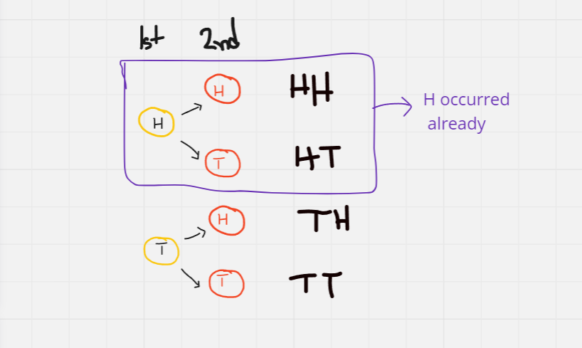
So this leaves us with the lower half portion, from where we need to calculate the probability of getting a H, because the first half does not matter anymore as we know a H occurred there. The denominator is not 4, it's 2 now. So the answer is 1/2

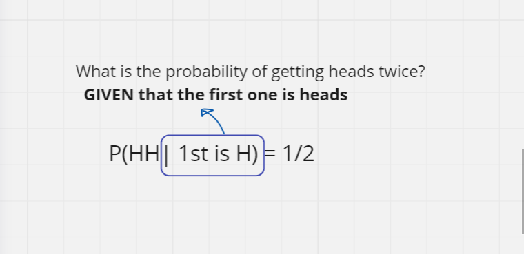
Question : What is the probability of getting heads twice? GIVEN that the first one is tails

Answer : Zero. Because if it lands on tails then there is no chance of occurring two heads. The denominator becomes two but the numerator is now zero as no heads landed.

Remember the product rule? It was P(A∩B) = P(A) × P(B). But it's only for independent events. For Dependent Events (The occurrence of one event affects the probability of the other) the joint probability is the product of the probability of the first event and the conditional probability of the second event given the first.

P (A∩B) = P(A) × P(B|A) The General Product Rule

When they are dependent, probability of B given A P(B|A) is equal to being probability of B P(B) as A doesn't makes any difference. But in the general case, it's P of A times P of B given A, and this rule works every time

Conditional Probability - Part 2

Question : In a school there are 100 kids, where 50 like footbal and 50 don't. There are two rooms where in room 1 there is a TV playing a match and in room 2 there is a TV playing a movie unrelated to soccer. Each room fits exactly 50 kids. How many kids that like soccer you expect to be in room 1? Note: The kids have the liberty to choose any room.

Answer : We can guess that all the 50 kids who likes soccer went to the room where the TV is showing a soccer match. It may not happen but we can guess. So, these two events soccer and room one are dependent. In the previous example, we split 50/50 randomly - that was independent.

Question : In a school, 40 of the students plays soccer and 60 don't. 80% of the 40 students wear running shoes. How many kids plays soccer and wear running shoes?

Answer : 80% of 40 is 32. And 32 is the range for how many students wear running shoes and likes soccer.

P (soccer and running shoes) => P (S∩R) = P(S) × P(R|S) = 0.4 x 0.8 = 0.32

Now, what if the probability of wearing running shoes while not liking soccer is 50% (among the kids who hates soccer, half of them wears running shoe) -

P (not soccer and running shoes) - ?

P (not S∩R) = P(not S) x P(R | not S) = 0.6 x 0.5 = 0.3

Bayes Theorem - Intuition & Formula

Bayes' theorem is a fundamental concept in probability theory that tells how to update the probability of hypothesis based on new evidence. It combines the prior knowledge with the new data to give an updated probability.

The formula for Bayes' theorem is:

P(A|B) = { P(B|A) x P(A)} / P(B)

To understand Bayes' theorem intuitively, let’s consider an example involving medical testing.

Example: Disease Testing

Suppose you are tested for a rare disease. Here are some probabilities :

• Prior Probability P(A) : The probability of you have the disease before any testing is 1% (0.001)

• Complement of Prior Probability P(A') : The probability that you don't have the disease is 99% (0.99)

• Likelihood P(B|A) : The probability that the test correctly dragonized the disease (true positive rate) is 99% (0.99)

• False Positive Rate P(B|A') : The probability that the test says you have the disease when you don't have is 5% (0.05)

Given the values:

• P(A, sick) = 0.01 (prior probability of having the disease)

• P(B|A, tested sick| sick) = 0.99 (probability of testing positive if you have the disease)

• P(B|A' , tested sick| not sick) = 0.05 (probability of testing positive if you don't have the disease)

• P(A' , not sick) = 0.99 (probability of not having the disease)

Calculating the marginal probability P(B):

P(B) = P(A)*P(B|A) + P(A')*P(B|A')

P(B) = (0.01*0.99) + (0.05*0.99) = 0.0549

Putting all the values in the Bayes formula, to find you have the disease given that you tested sick, we get P(A|B) = 0.1667 or, P(sick| dragonized sick) = 16.67%.

Bayes Theorem - Spam example

Let's apply Bayes' theorem to a spam email detection example. This is a practical use case often used in email filtering systems.

Problem Setup:

• S : Spam email

• W : The email contains a word "Hello"

Given:

• The probability that any given email IS SPAM , P(S) = 20% (0.20).

• The probability that any given email is NOT spam, P(S') = 80% (0.80).

• The probability that the word "Hello" appears in a spam email, P(W|S) = 70% (0.70)

• The probability that the word "Hello" appears in a non-spam email, P(W|S') = 5% (0.05)

We want to find the probability that an email is spam given that it contains the word "Hello", P(S|W) [WE ONLY CARE ABOUT EMAILS THAT CONTAINS THE WORD "HELLO"]

Formula : P(S|W) = { P(W|S) * P(S) } / P(W). In other words, P(spam|Hello) = spam and hello / all hello

P(W) = P(S)*P(W|S) + P(S')*P(W|S') = 0.2*0.7 + 0.05*0.8 = 0.18

P(S|W) = (0.7*0.2)/0.18 = 0.7778

Prior Probability

The prior probability, P(A) is our initial estimate of the probability of an event A before new evidence is taken into consideration. It is basically based on previous evidence, knowledge and experience.

Posterior Probability

The posterior probability, denoted as P(A|B), represented the new updated probability of an event A after taking new evidence B into consideration. It's basically the combination of prior probability and the likelihood of the new evidence to provide an updated probability.

Lesson 2 - Probability Distribution

Let's start the 2nd lesson of week 1!

Random Variable

Random variable is a variable that stores values which are outcomes of different random phenomenon. It is used in probability theory and statistics in order to model uncertainty and various experiments. Random variables can be classified into two main types: discrete and continuous.

Probability Distributions (Discrete)

A probability distribution describes how the values of a random variable are distributed. Variables that takes countable type of data are called discrete variable. For example, number of heads when flipping three coins, number of car passing in an hour, number of student present in a class and so on

Key Functions in Probability Distributions:

Probability Mass Function (PMF):

• Used for discrete random variables.

• The PMF P(X=x) gives the probability that the random variable X equals a specific value x

• Example: For a fair six-sided dice, P(X=x) = 1/6 for x = 1,2,3,4,5,6.

• Condition : Sum of all PMF must be 1

Binomial Distribution

What is the probability if you flip 5 coins, two of them land in heads?

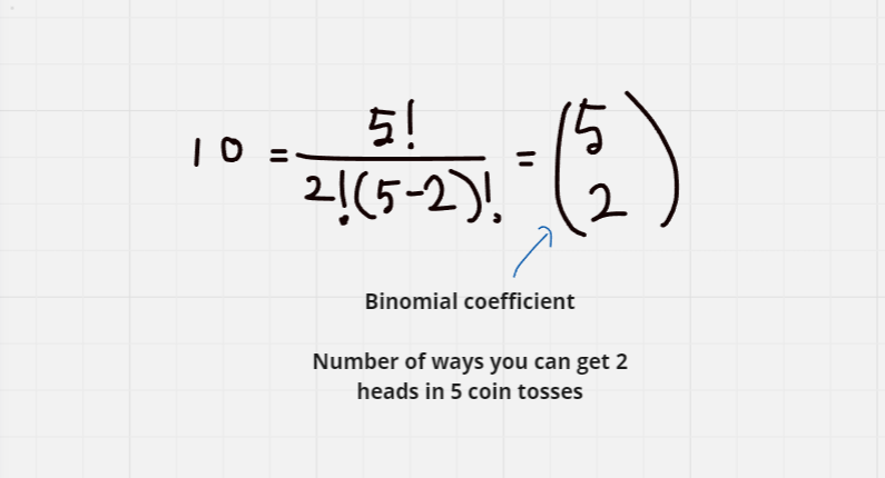
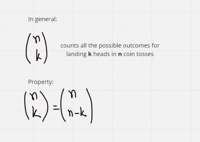
Question :

General PMF for X: number of heads in 5 coin tosses?

Coin has P(H) = p

Event: X = x: x heads in 5 tosses

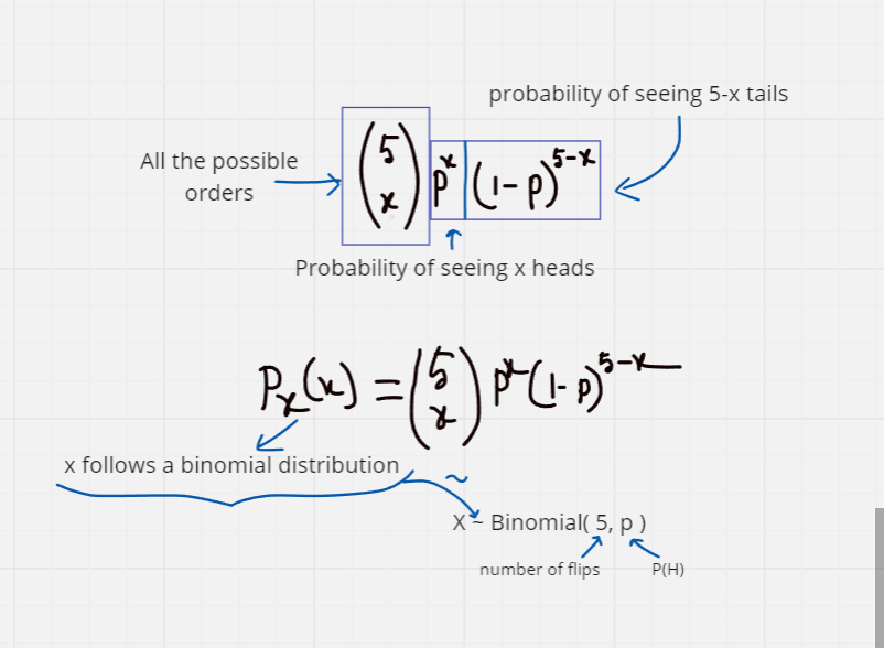
Key Characteristics of the Binomial Distribution

1. Number of Trials (n):

   • The fixed number of independent trials or experiments.

2. Probability of Success (p):

   • The probability of success on a single trial.

3. Number of Successes (k):

   • The number of successes in n trials.

Bernoulli Distribution

The Bernoulli distribution is a simple probability distribution for an event that has exactly two outcomes: success (1) and failure (0).

Parameter: p(the probability of success).

PMF:

• P(X = 1) = p [X = Number of heads]

• P(X = 0) = 1 − p

Example:

• Coin Toss:

  • Success (heads) with p=0.5.

  • Failure (tails) with 1−p=0.5

Probability Distributions (Continuous)

In a discrete distribution, the events always formed a list. But continuous distribution can't be listed. For example, waiting for the bus, because I can wait 5mins for the bus, or 6 mins, or pi mins or 20 mins, there are infinitely possible values - all these numbers can't listed. So when we have a listed events : it's a discrete probability distribution and when there is an interval : it's a continuous probability distribution.

What is the probability that you will wait exactly one minute for a call? Answer : Zero. Because there are uncountable amount of time a call could last.

Unlike discrete distribution, continuous distribution can take any value within a certain range. The probability of a random variable value falling into a interval is given by the area under the curve of it's probability density function (PDF)

Example: The exact height of a person can be any value within a range (e.g., between 150 cm and 200 cm). The probability of the height being exactly 170 cm is zero, but we can calculate the probability that the height falls within a specific interval, such as between 170 cm and 175 cm.

Probability Density Function

Let's say, a group of people eats apple in a day with equal probability at any qty between 0-5. If we divide the area in five parts, the probability of eating any qty apple is same. Given the info, what is the probability that a person eats apple in a day is between 2-3?

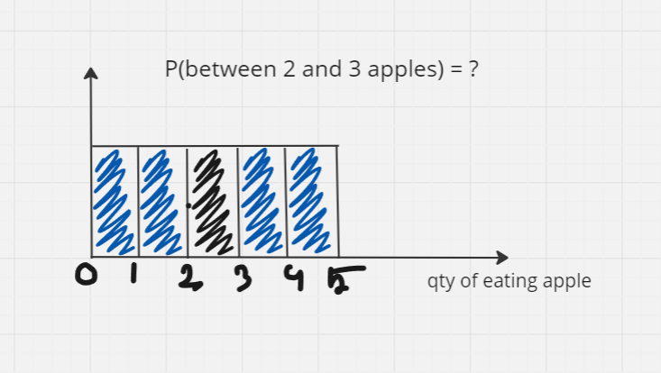
Well, if you say 20% or one fifth, than you are correct.

Now let's split it into 10 small intervals. What is the probability of eating 2-2.5 apples in a day?

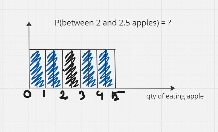
it's 10%, because it's 1/10th. Look carefully, the height of the columns does not change, but the width of the columns were halved, therefore the probability have been halved too. So, here we can't think of heights, we need to think of areas instead.

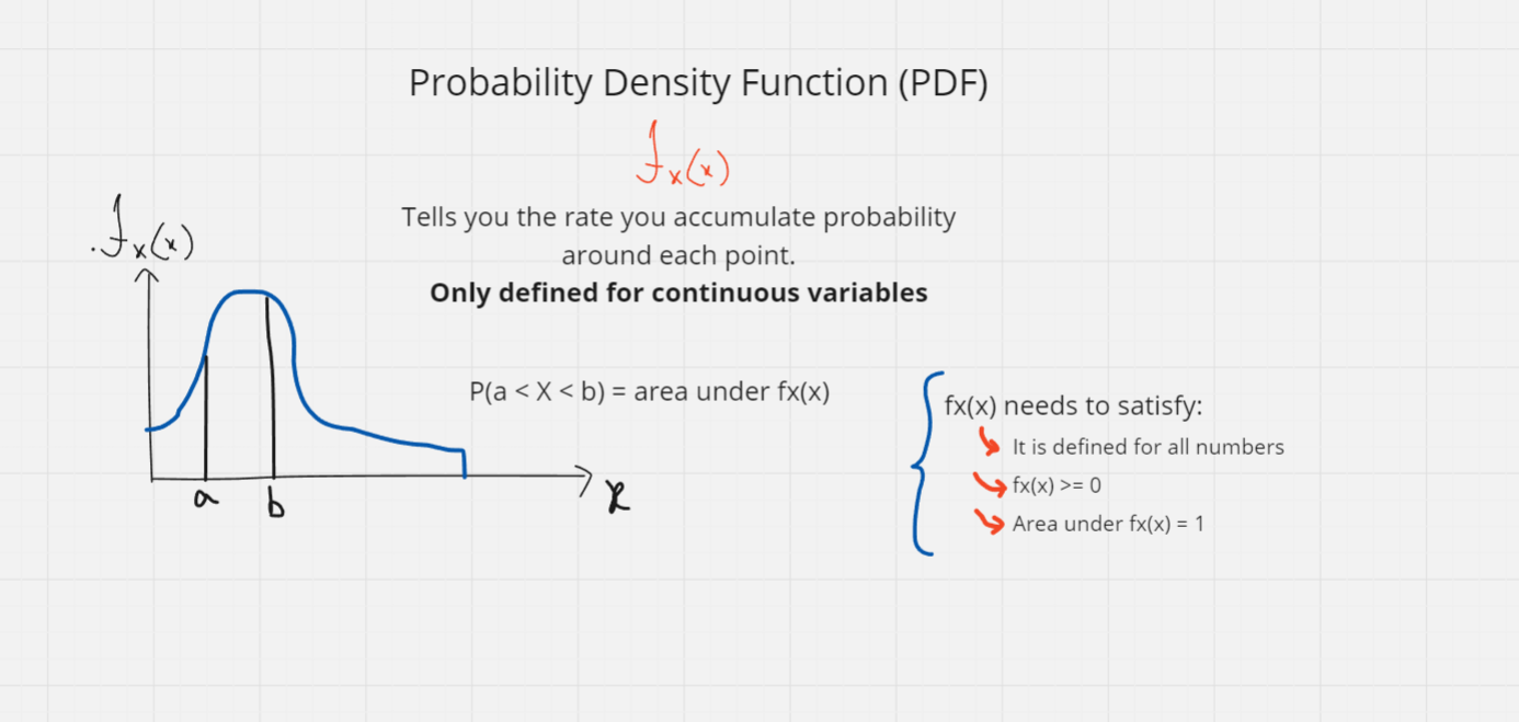
The area under the curve has to be 1. This restriction comes because the area under the curve is simply the probability of all possible outcome and the addition of the outcomes must be one. Also, fx(x) needs to be greater than zero, otherwise negative possibility will appear which is not possible.

Cumulative Distribution Function

The Cumulative Distribution Function (CDF) of a continuous random variable is a function that says the probability, that the variable contains a value which is less than or equal to another specific value (x)

For a random variable, X, the CDF, denoted as F(x) is: F(x) = P ( X <= x)

Points to Remember :

1. The CDF ranges from 0 to 1

2. CDF never decreases as x increases

3. The function is continuous from every point to the right, always positive and increasing

4. Endpoints can be at infinity

The CDF shows how much probability a variable has gained until a certain value.

Uniform Distribution

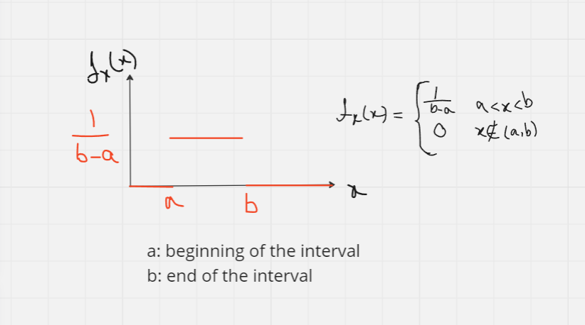
The uniform distribution is useful for modeling situations where all outcomes within a specific range are equally likely, combination of constant PDF and linear CDF

Gaussian or Normal Distribution

The normal distribution or the Gaussian distribution is one of the most popular distribution in probability distributions in statistics. It describes how values of a variable are distributed.

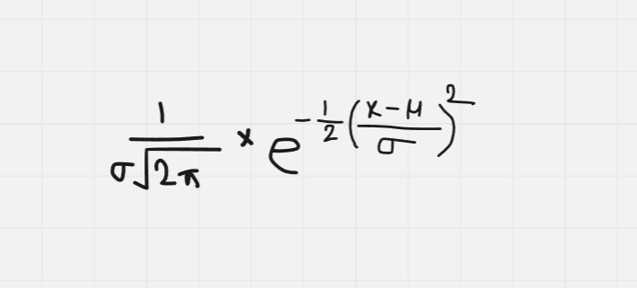
Here,

• μ is the mean (average) of the distribution (Center of the bell curve)

• σ is the standard deviation (Spread of the bell)

• e is the base of the natural logarithm.

• π is the constant pi

• Symmetric

• Normal Distribution Notation : X ~ N( μ , σ ^2)

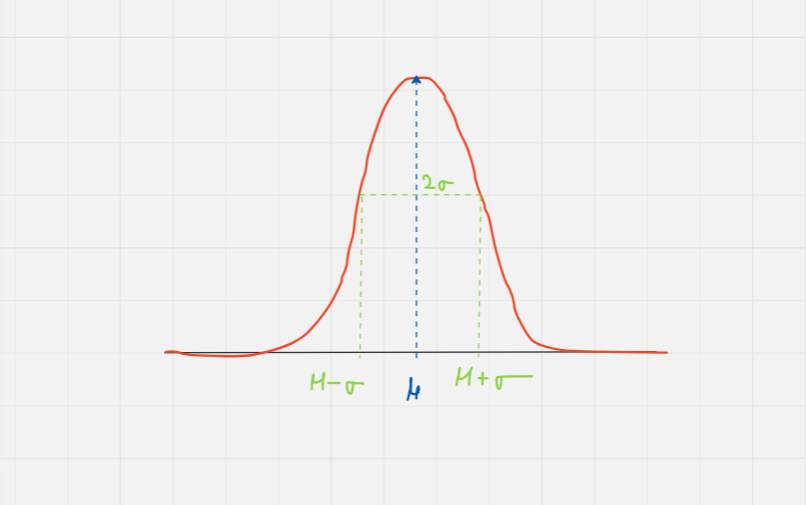
The normal distribution is a fundamental concept in statistics with wide-ranging applications in various fields. It is defined by bell shaped curve, characterized by the mean μ and standard deviation, , and used to model natural and human phenomena. I would like to encourage to go through Normal Distribution website for better understanding.

Yayyy! We have finished week -1! To sum up, we have learned probabilities, random variables and probability distribution. In the next blog, we are going to dive in depth of week - 1.

Don't forget to stay hydrated!!