Data Science - introduction to the world of data
 Debanjan Chakraborty
Table of contents
- Introductions:
- Prerequisites of Data Science:
- Data science life cycle:
- Components of Data science:
- Tools and skills used in data science:
- Solving questions with data science:
- Algorithms used in Data Science:
- Top 5 Python libraries for Data science:
- Linear Regression Analysis:
- Logistic Regression Analysis:
- Confusion Matrix:
- Decision Trees:
- Random Forest:
- Support Vector Machines:
- K Means Clustering:
- Dimensionality Reduction:
- Thank You

Introductions:
Data science is the field of study that involves extracting knowledge from all of the data gathered. There is a huge demand for analysts who can convert data into competitive advantage. In Data science as a career, we will create Data driven business solutions and analytics. Here we will cover a detailed overview of data science as a whole.
Prerequisites of Data Science:
Non technical:
Curiosity: should have the ability to ask questions
Common Sense: Find new ways to solve a business problem
Communication skills: key trait for a data scientist to communicate the results
Technical:
Machine Leaning
Mathematical modeling
Statistics
Computer programming
Databases
Data science life cycle:
Business problem :
being curious and asking the question why? multiple times. Also known as concept study.
Data Acquisition:
Gather data from multiple sources like: Web servers, Logs, Databases, API's, Online Repositories, etc.
Data Preparation:
This step involves data cleaning(time consuming) and data transformation. Data cleaning removes inconsistent datatypes, missing attributes, Missing and duplicate values. In data transformation we modify the data based on defined magnitudes, tools like Talent and informatic are used here.
Exploratory data analysis:
The most crucial step in this process. With this we define and refine the selection of feature variables, that will be used in the model development. Not doing this step might lead to wrong selection of features and a faulty model of the data.
Data Modeling:
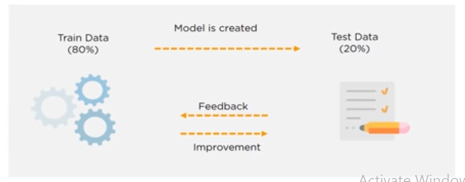
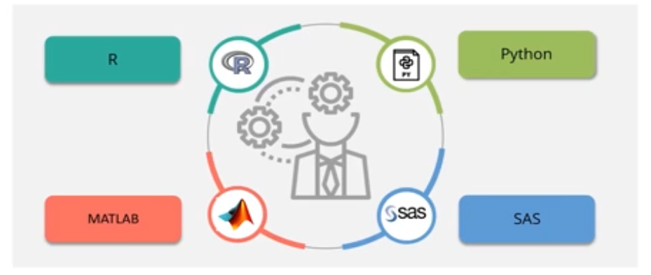
Now comes the core job of a data analyst, that is to repetitively apply diverse machine learning techniques to identify the model that best fits the dataset and the business requirement. Train the model on the dataset and test it. we can use tools like python, R and SAS.
Visualization and Communication:
Now we have to communicate the business findings in a simple and representable way using tools like Tableau, PowerBi and QlikView to create powerful reports and dashboards.
Deployment and Maintenance:
Involves testing of the model in the preproduction environment and then deploys it in the production environment. Creating repost on a regular interval to monitor the performance is crucial. Also known as Operationalization.
Components of Data science:
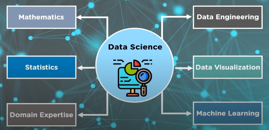
Out of all these Domain Expertise.
Tools and skills used in data science:
Data Analysis:
Skills: R, python, Statistics
Tools: SAS, Jupyter, R studio, MATLAB, Excel, Rapid Miner
Data Warehousing:
Skills: ETL, SQL, Hadoop, Apache Spark
Tools: Informatica/Talend, AWS redshift
Data Visualization:
Skills: R, Python libraries
Tools: Jupyter, Cognos, Tableau, RAW
Machine Learning:
Skills: Algebra, ML algorithms, Statistics
Tools: Spark Mlib, Mahout, Azure ML studio
Solving questions with data science:
| Possible Question | Desired Algorithm |
| How much or How many | Regression |
| Is it A or B | Classification |
| How is it organized | Clustering |
| How different is it? | Anomaly detection |
| What to do next? | Reinforcement Learning |
Algorithms used in Data Science:
Linear Regression
Logistic Regression
Decision tree
K nearest Neighbors
K Means Clustering
Hierarchical clustering
DBSCAN
Principal component Analysis
Support Vector Machines
Naïve Bayes
Top 5 Python libraries for Data science:
Tensor Flow:
Used for high performance numerical calculations
Used across various scientific domains
Framework that defines and runs computations with the help of tensors(partially defined computational objects)
Features:
Better computational graph visualizations
Reduces errors by 50-60% in Neural machine translations
Parallel computing to execute complex models called Pipeline
Seamless library management
Applications:
Speech/Image recognition
Text based applications
Time Series
Video Detection
NumPy:
stands for Numerical python
general purpose array processing package
Contains powerful N dimensional array objects used for computation
Features:
Provides fast and precompiled functions for numerical routines
Array oriented computing for better efficiency
Supports object oriented approach
Compact and faster computations with vectorization
Applications:
Data analysis
Create powerful N- dimensional array
forms the base for other libraries like SciPy, scikit-learn
Replacement for MATLAB when used with SciPy and matplotlib
SciPy:
stands for scientific python
used for scientific and technical computations
provides many used friendly routines for scientific computation
Features:
Collection of mathematical algorithms and scientific functions built on NumPy extension
high level commands and classes for manipulating and visualizing the data
multidimensional image processing with scipy.ndimage
includes functions for computing integrals numerically, Solving differential equations, Optimization, etc.
Applications:
Multidimensional image operations
solving differential equations and Fourier transforms
Optimization algorithms
Linear Algebra
Pandas:
Stands for python data analysis library
used for data analysis and cleaning
provides fast, flexible and expressive data structures designed to work with easily and intuitively
Features:
Eloquent syntax and rich functionality
Apply() enables you to run a function across a series of data
High level abstraction
High level data structures and manipulation tools.
Applications:
General data wrangling and data cleaning
ETL jobs and data storage
used in wide variety of academic and commercial domains, including statistics, etc.
Time- series specific functionality
Matplotlib:
plotting library for python
used for data visualization
provides and object oriented API for embedding plots into applications
Features:
as usable as Matlab but with an added advantage of being free and open source
supports dozens of backends and output types
pandas itself can be used as wrappers around matplotlib's API
smaller memory consumption and better runtime behavior
Applications:
Correlation analysis of variables
visualize 95% confidence intervals of the models
outlier detection
visualization of distributions to get instant insights
Linear Regression Analysis:
It is a statistical model used to predict the relationship between independent and dependent variables.
They Examine 2 factors:
Which variables in particular are significant predictors of the outcome variable,
How significant is the regression line to make predictions with highest possible accuracy.
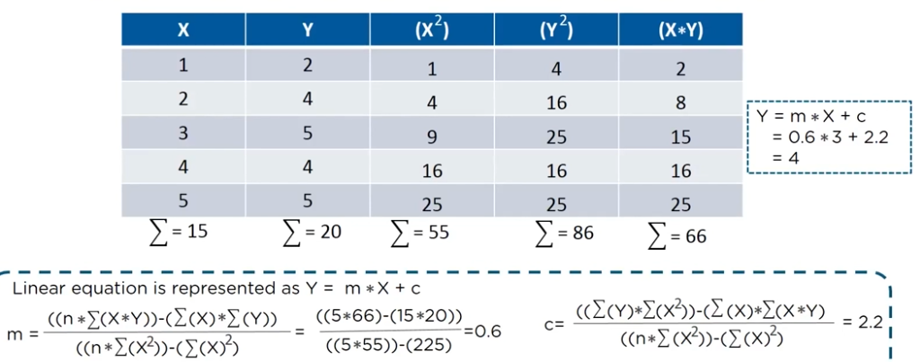
The simples form of simple linear regression equation with one dependent and one independent variable: y = mx + c
where y->independent variable; x->dependent variable; m->slope of the line and c->coefficient of the line
m=(y2-y1)/(x2-x1)
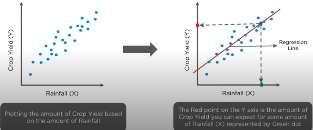
Intuition behind the regression line:
let us consider a dataset with 5 rows and find out how to draw the regression line.
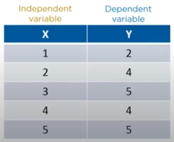
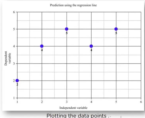
now we plot it on the graph:
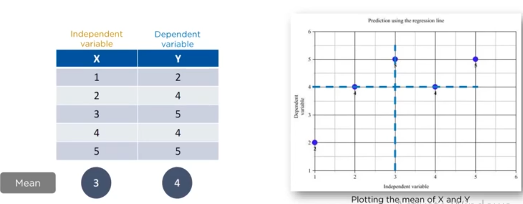
now we find the mean and plot it on the graph:
now we find the m and c value in the line equation:
now the line equation is the predicted values of y which we plot on the graph:
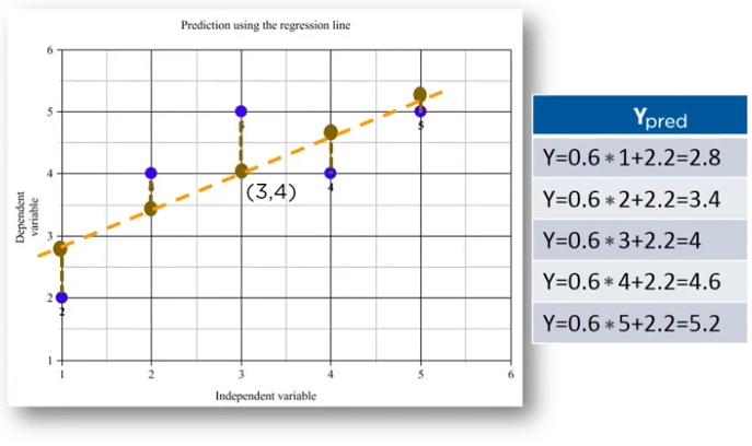
now we calculate the squared errors with respect to the actual points:
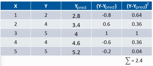
now based on this we Minimize the distance between the line and the points with techniques like Sum of squared error, Sum of absolute errors, Root mean squared errors, etc.
now in real world there are many values rather than the 2 we took as example, for understanding that we go into Multiple linear regression.
Multiple Linear Regression:
- In simple linear regression we take y = mx + c, but in multiple linear regression, we take y = m1x1 + m2x2 + ..... + mnxn + c.
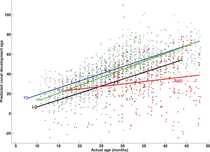
Implementation of linear regression:
we use the metric root mean squared error to access the model trained.
Logistic Regression Analysis:
It is a classification algorithm, used to predict binary outcomes for a given set of independent variables, the dependent variable's outcome is discrete.
for example if we want to predict whether a car will break down with a factor of its time from the last servicing:
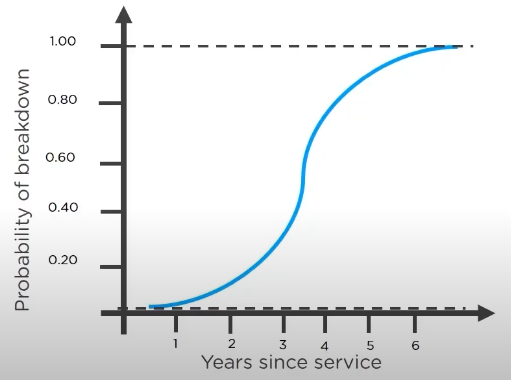
now the logistic regression graph looks like:
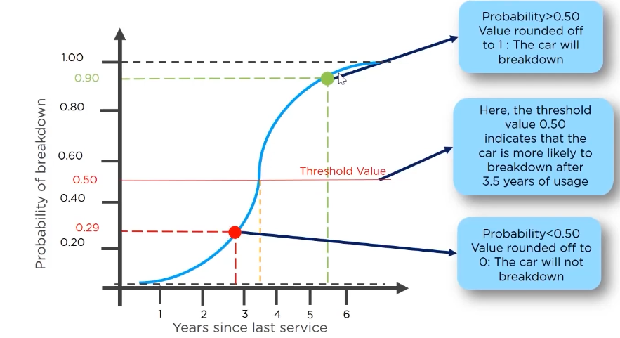
Now comparing linear and logistic regression:
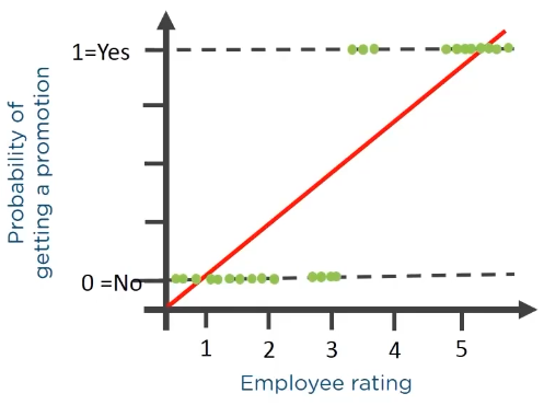
it helps to find the relation between the independent variable and the dependent variable, both of which are continuous
e.g. determine the salary hike of an employee based on their ratings
if we use linear regression for the logistic graph then there will be very high RMS error, shown in the figure below:
Maths behind logistic regression:
In logistic regression we find the odds of an event happening:
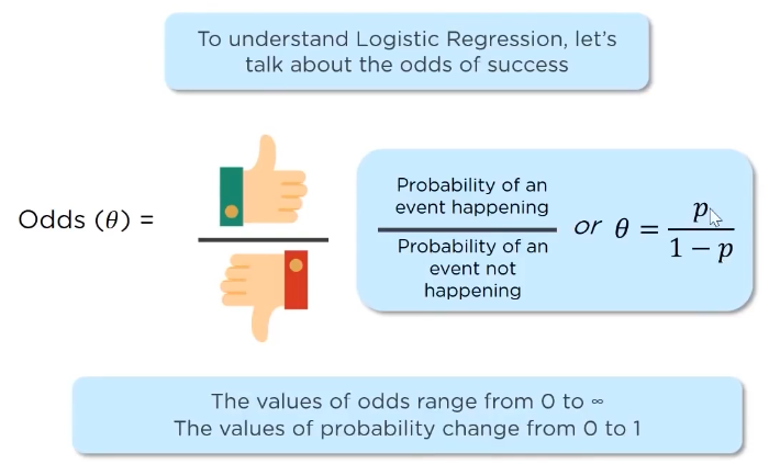
now this will how the line equation will look:
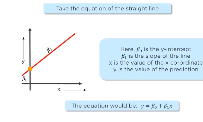
now if we take the odds equation and take log on both sides, then:
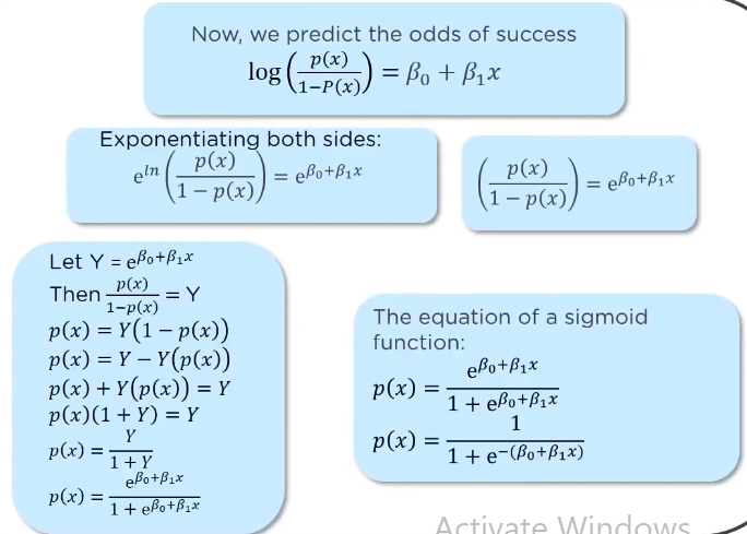
And the term LOGistic regression by the fact that we are using log on both sides,
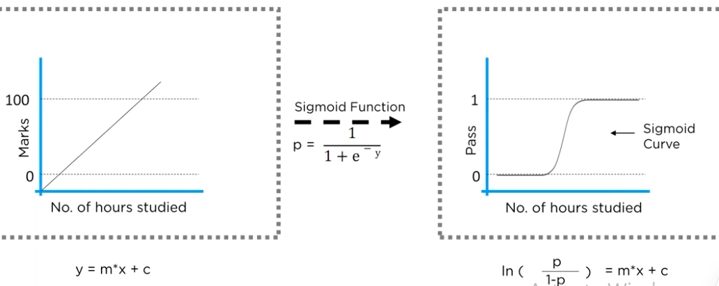
hence the equation of logistic regression is the sigmoid function.
when plotted then the line equation would look like:
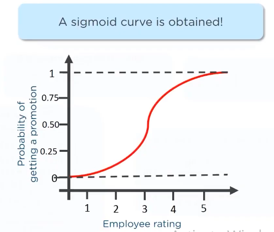
Comparing logistic and linear regression:
| Linear Regression | Logistic Regression |
| Used to solve regression problems | Used to solve classification problems |
| the response variables are continuous in nature | The response variable is categorical in nature |
| It helps estimate the dependent variable when there is a change in the Independent variable | It helps calculate the possibility of a particular event taking place |
| It is a straight line | It is an S -curve(Sigmoid) |
Applications of Logistic Regression:
Whether it is going to rain or not, sunny or not, snow or not(if we want to predict the temperature then the problem also has linear regression in it)
Image categorizations
check survival rate of a patient based on multiple tests
Practical Example: predict the number in the image
Confusion Matrix:
Classification models have multiple output categories, most error measures will tell the total error in the model, but we cannot use it to find out individual instances of errors in our model, for that we use the confusion matrix.

During classification we also have to overcome the limitations of accuracy. Accuracy can be misleading for classification problems, if there is a significant class imbalance, a model might predict the majority class for all cases and have a high accuracy score.
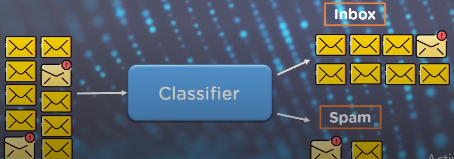
for example if we see the classifier, it gives 8/10 instances, so is the accuracy 80 percent?
A confusion matrix presents a table layout of different outcomes of prediction and results of a classification problem and helps visualize its outcomes.
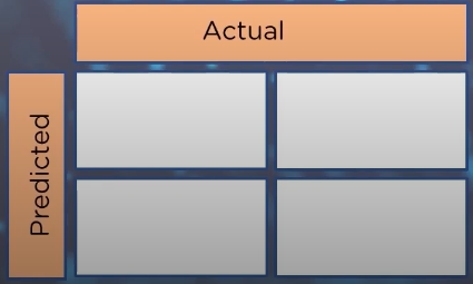
The confusion matrix helps us identify the correct predictions of a model for different individual classes as well as the errors.
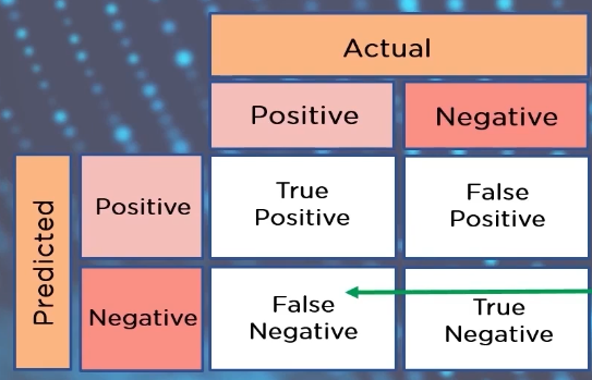
Confusion matrix metrics:
there are 4 major metrics:
Accuracy
Precision
Recall
F1-Score
Accuracy:
used to find the portion of correctly classified values, it tells us how often our classifier is correct
it is the sum of all true values divided by total values:

Precision:
used to calculate the models ability to classify positive values correctly,
it answers the quest: "When a model predicts a positive value, how often is it right?"
it is true positives divided by total number of positive predicted values:

Recall:
used to calculate the model's ability to predict positive values.
"how often does the model actually predict the correct positive values?"
it is true positives divided by total number of actual positive values:

F1-Score:
it is the harmonic mean of recall and precision
useful when you have to take both recall and precision into account:

Decision Trees:
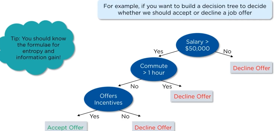
Decision tree is a tree shaped diagram used to determine the course of action, each branch determines a course of action and decision, occurrence or reaction.
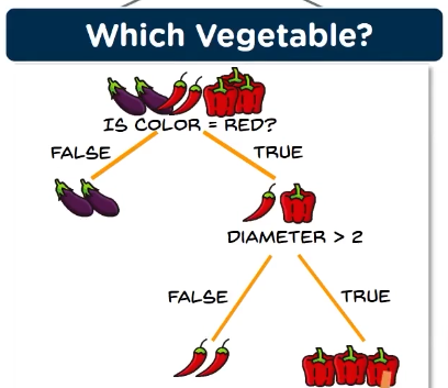
Problems that decision tree can solve:
Classification:
classification tree will determine a set of logical if-then conditions, to classify the problems.
for example, discriminating between three types of flowers based on certain features.
Regression:
regression tree is used when the target variable is numerical or continuous in nature,
We fit the regression model to the target variable using each of the independent variables, each split is made based on the sum of squared error
Advantages of the decision tree:
Simple to understand, interpret and visualize.
little effort needed to prepare data.
Can handle both numerical and categorical data.
Non linear parameters don't effect its performance.
Disadvantages of the decision tree:
overfitting occurs when noise gets captures by the algorithm
the model can get unstable due to small variance in data
A highly complicated decision tree tends to have a low bias which makes it difficult for the model to work with new data.
Important terms in decision trees:
Entropy:
it is the measure of randomness or unpredictability in the dataset,
example:
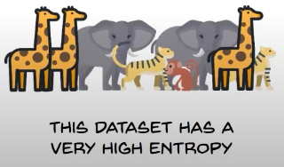
Now we split the groups: then we come across the Information Gain:
It is the measure of decrease of entropy after the dataset is split,
example:
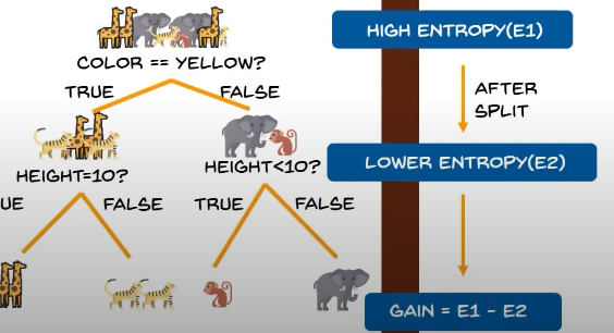
Leaf node:
it carries the classification or the decision
example:
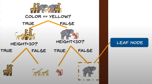
Root node:
- The topmost decision node
How does a decision tree work?
problem statement: classify the different types of animals based on their features using decision tree.
initial dataset:

we can use the features:
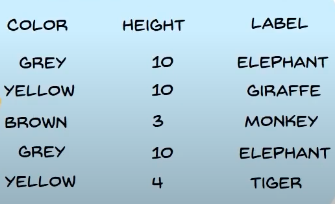
we calculate the entropy of the root node:

the numbers are:
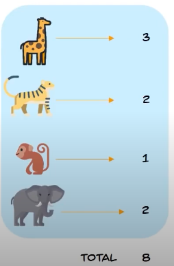
the entropy calculation is:

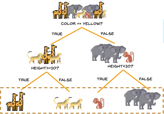
if we the information gain, the condition that gives us the maximum information, here "yellow" from the condition:
then we take the height as the condition and we get the decision tree:
Random Forest:
let us assume 3 decision trees:
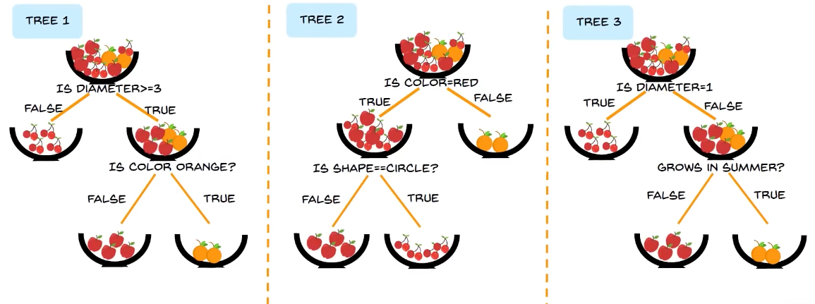
now let's try to classify this fruit:

now we can see these are the features of the object:

then we parse the decision trees:
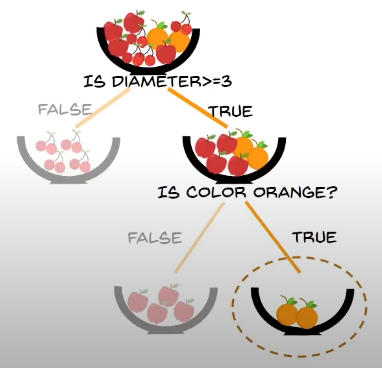
tree 1 classifies the fruit as orange
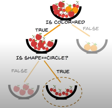
tree 2 classifies the fruit as cherry
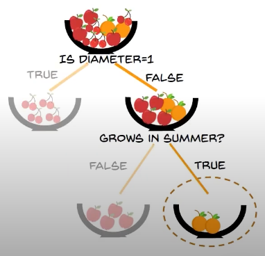
tree 3 classifies the fruit as orange
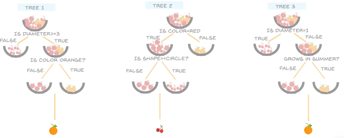
so out of 3 trees, 2 give orange, so the unknown object is classified as orange

Support Vector Machines:
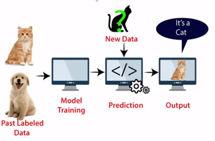
SVM is a non-linear supervised learning method that looks at data and sorts it into one of the two categories
for example, how SVM works:

the goal of SVM is to create the best line or decision boundary, called the hyperplane.
it can segregate n-dimensional space into classes so that we can easily put new data point in the correct category in the future.
SVM is divided into 3 types:
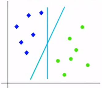
Linear SVM:
used for linearly separable data
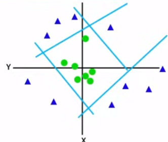
Non-linear SVM:
used for non-linearly separable data
How SVM works:
SVM chooses the extreme points or vectors that help in creating the hyperplane called the Support vectors.
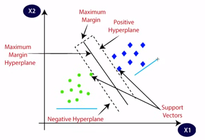
SVM works like:
Kernel:
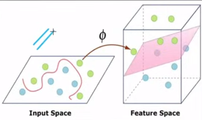
in case of non-linear SVM, kernel enables SVM to convert original feature space into higher dimensional space
types of support vector kernel:
Linear kernel:
simplest kernel function
performs linear transformation on input data without introducing any new dimensions
used for text classification tasks
Polynomial kernel:
introduces new dimensions by computing all possible polynomials up to specified degree of original features.
Gaussian Kernel:
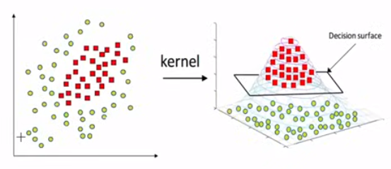
Also known as Radial Basis Function kernel(RBF)
maps the data into infinite dimensional plane where each data point is represented by a gaussian function.
kernel functions for SVM:
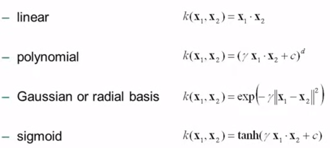
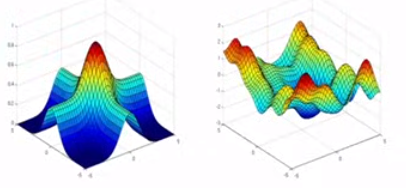
Gamma parameter controls the influence of each training example on the decision boundary, x1 and x2 represent the data we are trying to classify
the hyperplane is always at 1 less dimension than the feature space.
if there are three features then hyperplane is a 2D plane otherwise for 2 features it is a straight line
We always create a hyperplane that has maximum margin that is maximum distance between the data points
Properties of SVM:
Maximal margin: find hyperplane that maximizes the distance between the hyperplane and the closest data points
Non linearity of kernel: kernel transform data to higher dimensional feature space where linear decision boundary can be found
Support vectors: these are the data points that are closest to the boundary
Sparsity: SVM has a sparse solution that is the decision boundary is determined by only a small number of support vectors rather than the entire training dataset
Versatility: SVM can be applied to both classification and regression
Control of complexity: only algorithm that gives the freedom to control the complexity through the choice of hyperparameters.
Issues:
scalability with large datasets
lack of probabilistic interpretation
Imbalanced data
Interpretability
K Means Clustering:
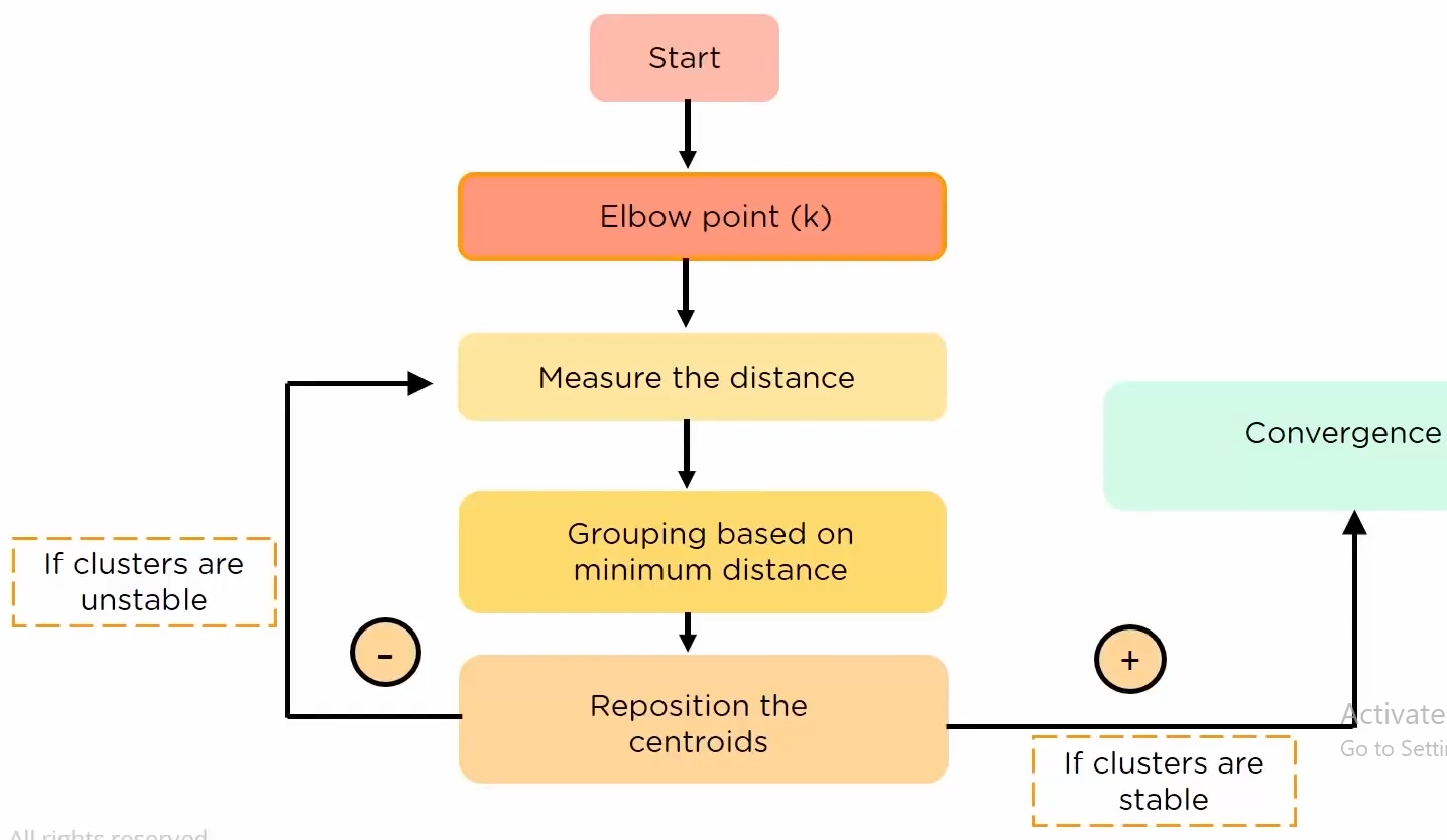
It is an unsupervised learning algorithm, where we group the object of similar nature into a cluster, where k is the number of clusters
Initially we allocate k centroids randomly(not necessarily the actual centroid of the cluster)
then we determine the distance of each and every point from that centroid and assign the near points to the corresponding nearest centroid.
Then the actual centroid is calculated, and then step 2 is repeated till there is no change in the centroid which will mean that the algorithm has converged
clustering and its types:
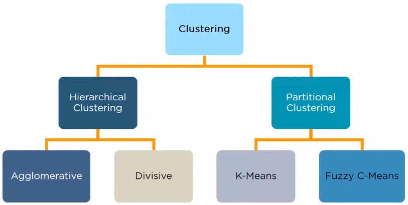
Hierarchical: clusters have a treelike structure.
Agglomerative: Bottom-up approach where we begin with each element as a different cluster and merge them into successive larger clusters.
Divisive: Top-down approach where we begin with a single cluster containing all the elements and we divide it into successive smaller clusters.
K-Means: divide the objects into clusters such that each object is in exactly one cluster.
Fuzzy C-Means: divide the objects into clusters but objects can be in multiple clusters.
Applications of K-Means Clustering:
Academic Performance
Diagnostic system
Search Engines
Wireless Sensor Network's
Distance Measures:
distance measure will determine the similarity between two elements and it will influence the shape of clusters.
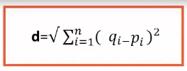
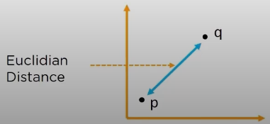
Euclidean distance measure:
it is the distance between two points on a straight line
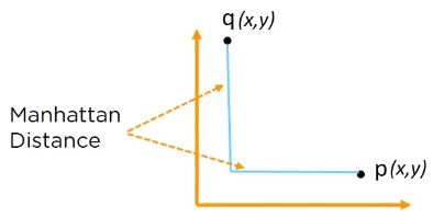
Manhattan distance measure:
it is the simple sum of horizontal and vertical components

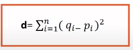
Squared Euclidean distance measure:
it is the same as the Euclidean distance formula, but instead of square root, we take square of the sum of differences.
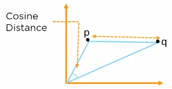
Cosine distance measure:
it measures the angle between the two vectors

How does K-Means Clustering work?
To choose an optimum number of clusters, we use the elbow method:
we calculate the WSS(sum of squared distance between each member of the cluster and its centroid)
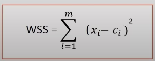
where xi = data point and ci = closest point to centroid
we then get the graph of k vs WSS
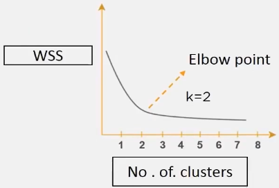
After the Elbow point, increasing the number of clusters does not make sense so the value of k at elbow point is taken as the best k value.
Dimensionality Reduction:
It refers to the techniques that reduce the number of input variables in a dataset.
less dimension's in a dataset means less computation or training time.
redundancy removed after removing similar entries from the dataset.
space required to store the data is reduced
makes the data easy for plotting in 2D and 3D plots
it helps to find out the most significant features and ignore the rest
leads to better human interpretation
Principal Component Analysis(PCA):
It is a technique used for reducing the dimentionality of datasets, increasing interpretability but at the same time minimizing information loss.

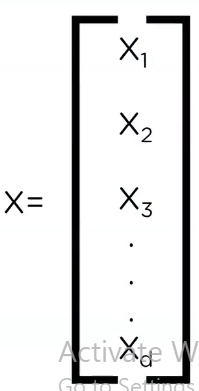
In simple terms of operation, in PCA we find out the best projection of the data points
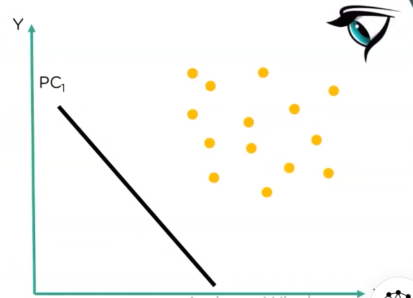
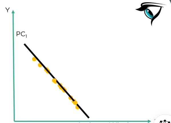
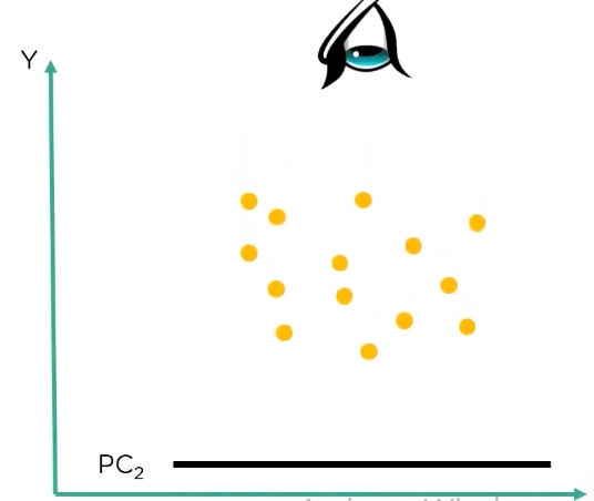
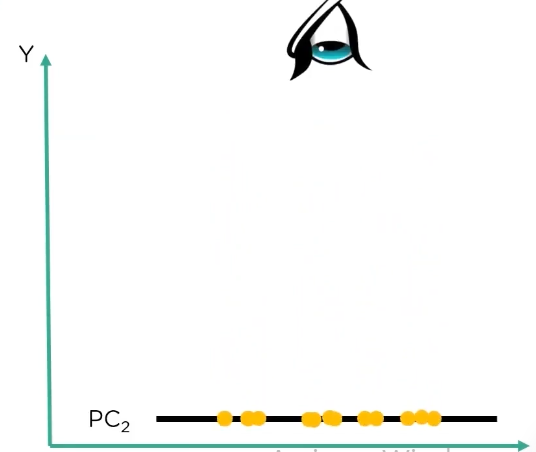
then we get two principal components:
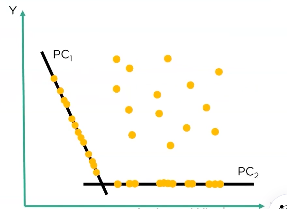
now if we compare the two principal components we extracted, we can see that PC1 has data points that are well spaced out
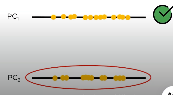
meanwhile if we see PC2, they are less spaced making further calculations difficult, so we go ahead with PC1
Important terminologies:
Views:
- the perspective through which data points are observed
Dimensions:
- number of columns in that dataset
Principal Component:
- new variables that are constructed as linear combinations or mixtures of the initial variables
Projections:
- the perpendicular distance between the principal components and the data points
Important Properties:
number of principal components is always less than or equal to the number of attributes.
principal components are orthogonal.
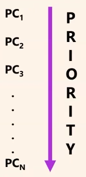
the priority of principal components decreases as the number of principal components increases.
How PCA works?

Standardization:
standardize the range of attributes so that each one of them lie within similar boundaries.
this process involves removal of mean from the variable values, and scaling the data with respect to the standard deviation

Covariance matrix computation:
used to represent the correlation between any two or more attributes in a multidimensional dataset.
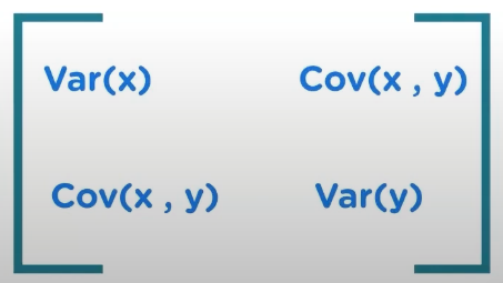
it has entries that are the variance and covariance of the attribute values.
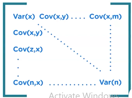
covariance matrix tells us how the two or more values are related:
positive covariance means there is a directly proportional relation between the two variables
negative indicates inverse relation
Eigen values and Eigen vectors:
they are the mathematical values extracted from the covariance table
they are responsible for the generation of new set variables from the old set of variables which further lead to the construction of PC
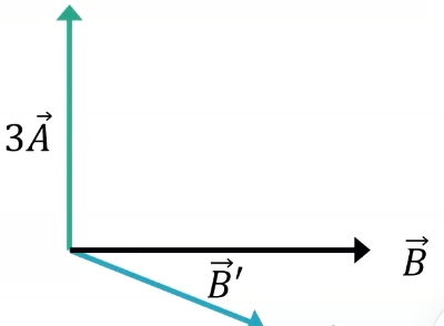
Eigen vectors do not change directions after linear transformation
Eigen values are the scalars or the magnitude of the eigen vectors
Feature Vectors:
A matrix that has the eigen vectors of the components that we decide to keep as columns.
Here we decide whether to keep or disregard the less significant PC that we have generated in the above steps.
Data science Interview Questions:
- List the differences between supervised and unsupervised learning:
| Supervised | Unsupervised |
| uses known and labeled data as input | uses unlabeled data as input |
| has feedback mechanism | has no feed |
| decision tree, logistic regression, support vector machines | k-means clustering, hierarchical clustering, apriori algorithm |
How is logistic regression done?
LR measures the relationship between dependent and one or more independent variables(features) by estimating probabilities, using the logistic sigmoid function:

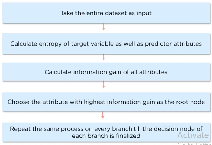
How to make a decision tree?
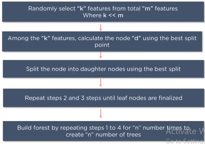
How to build a random forest model?
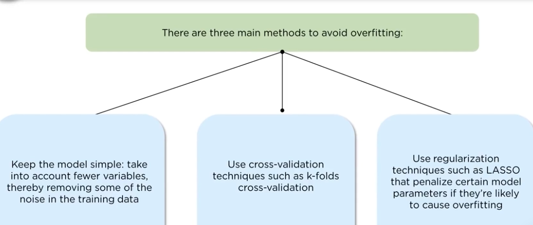
How to avoid overfitting in the model?
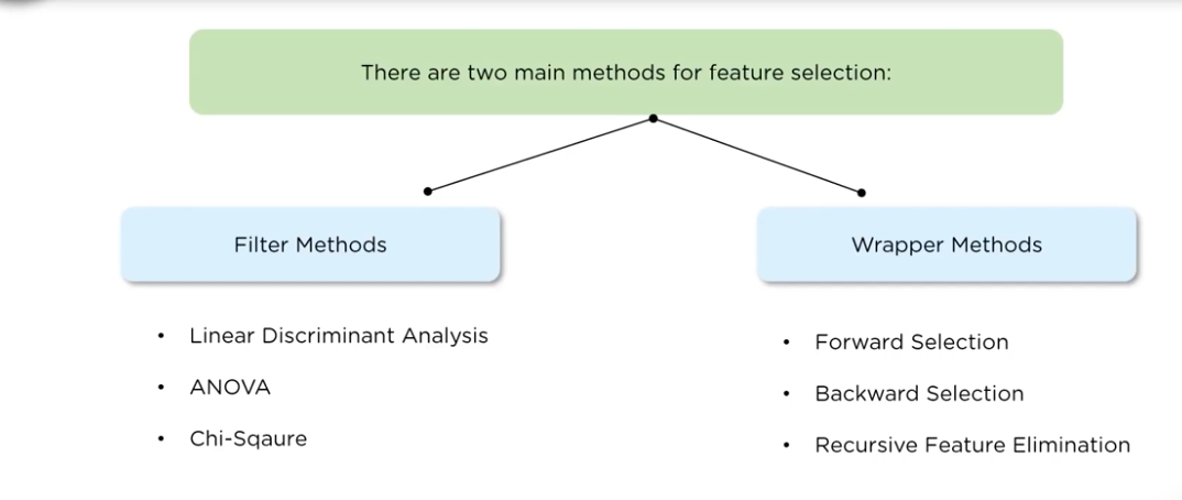
What are the feature selection methods to find the right variable?
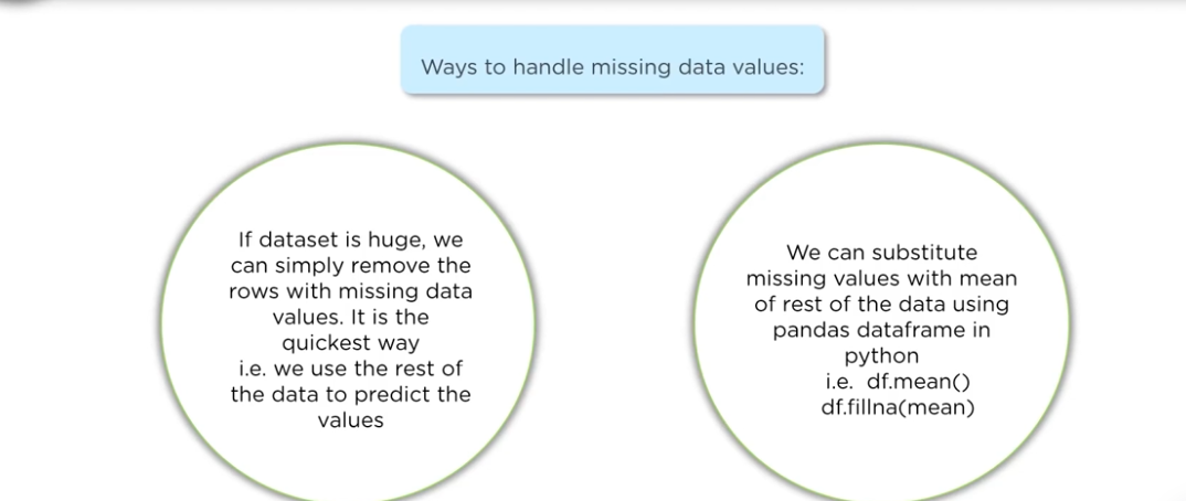
We are given a dataset of variables having more than 30% missing values, how to deal with them?
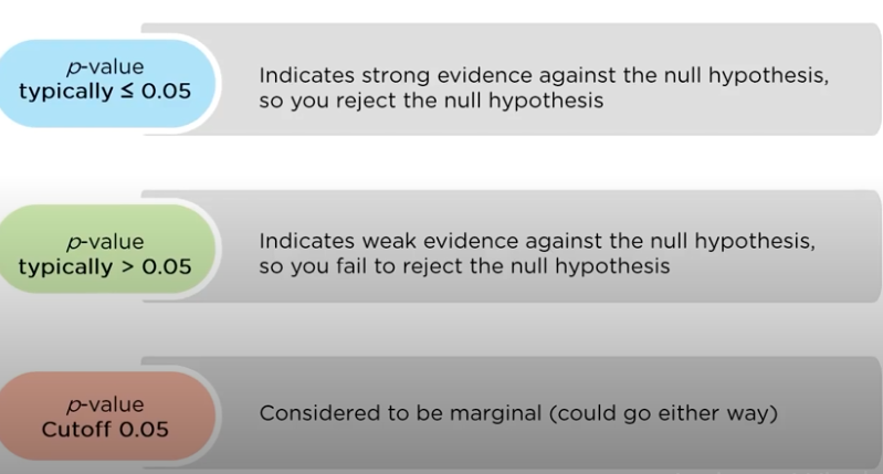
What is the significance of P-value?
How can outlier values be treated?
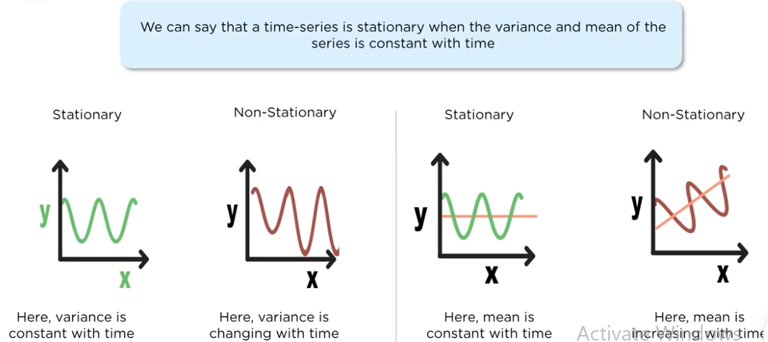
How can you day that the time series data is stationary?
"people who bought this, also bought this..." recommendations seen on amazon are a result of which algorithm?
which of the following algorithms can be used for imputing missing values of both categorical and continuous variable?
- K-NN
We want to predict the probability of death from heart disease based on three: risk factors: age, gender and blood cholesterol level. what is the most appropriate algorithm for this use case?
- logistic regression
After studying the behavior of the population, you have identified four specific individual types who are valuable to your study, you would like to find all individuals who are most similar to each individual type, which algorithm is most appropriate in this study?
- K-Means clustering
Thank You
Subscribe to my newsletter
Read articles from Debanjan Chakraborty directly inside your inbox. Subscribe to the newsletter, and don't miss out.
Written by

