I've been trying my hand at Transfer Learning and Fine Tuning for a while now. I decided to utilise it for a fun little project around F1.

I fine-tuned the EfficientNetB0 image classification model on a F1 car images dataset, so that, given an image of a F1 car, it would be able to tell the team that the car belongs to.

Here's everything on it.

P.S. here's a link to my notebook if you want to have a first hand look at the implementation.

(Mentions: This blog couldn't have been completed without the help ofAnkit Bhardwaj, a good friend and my batchmate from Thapar, and Kaggle UserAshwin Shetgaonkar, whose notebook proved to be extremely helpful. Check out their work on Kaggle!)

The Approach

Imports

This is the most basic, yet the most important step, the imports!

Here is everything you will need to build a Classifier using Transfer Learning.

import os
import numpy as np
import pandas as pd
import random
import tensorflow as tf
import matplotlib.pyplot as plt
%matplotlib inline
from sklearn.metrics import confusion_matrix
import seaborn as sns
from IPython.core.display import HTML,display
import tensorflow as tf
from tensorflow import keras
from tensorflow.keras import layers
from tensorflow.keras import mixed_precision
from shutil import copyfile
from PIL import Image

Data Handling

Before Transfer Learning, it is extremely crucial to prepare the data accordingly.

This includes loading the data correctly, preparing the data to be well suited to be an input to a pre-existing model, performing any Data Augmentation if required, etc.

Let's see how the dataset for this project was handled.

Loading The Data

I used the data available in this github repository. The data is structured into 3 parts.

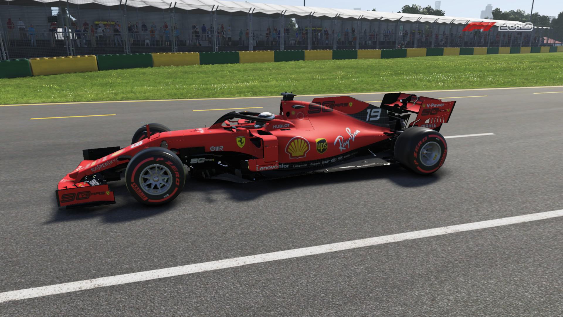
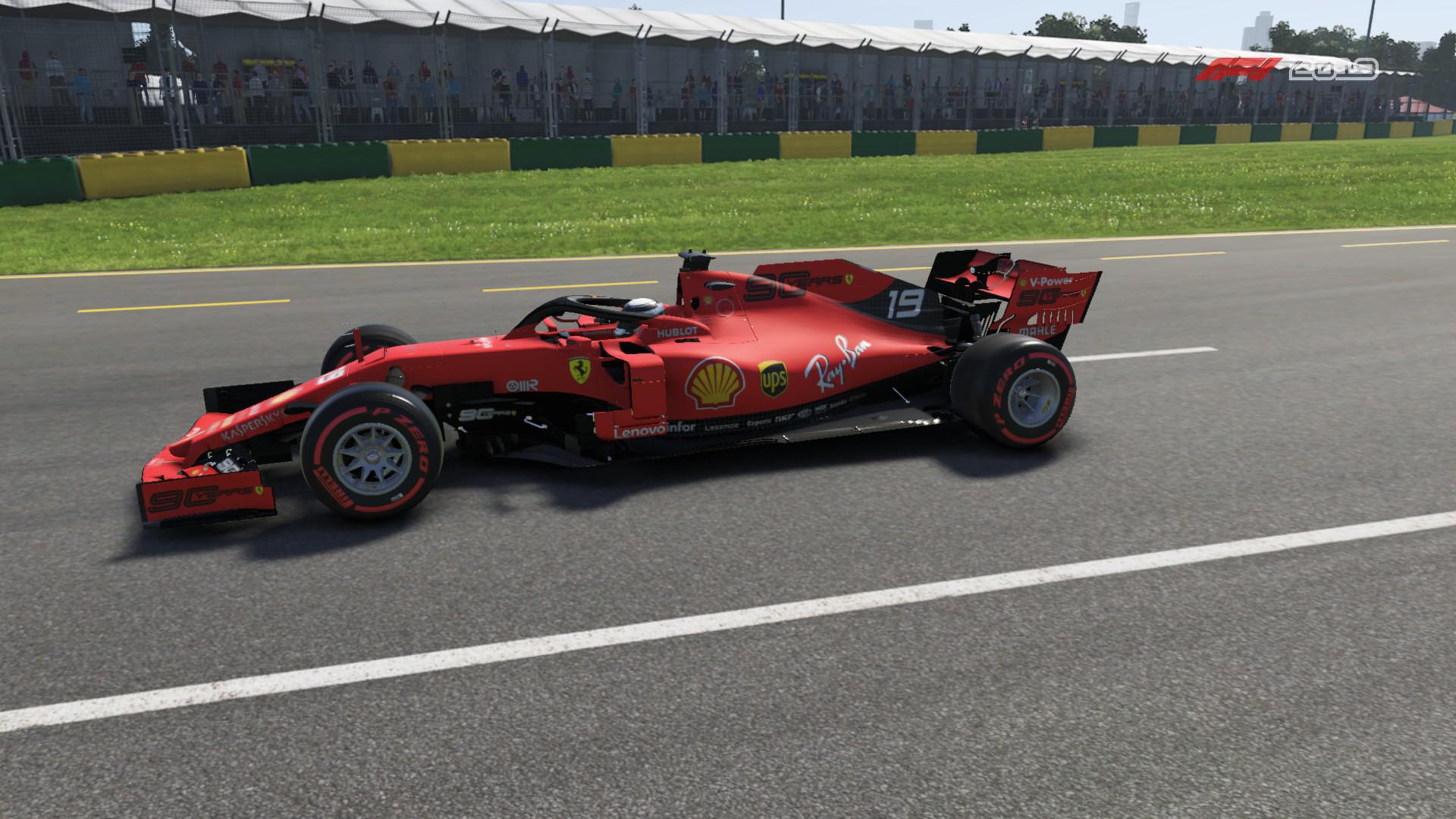
1. Train: Contains 10 folders of 10 F1 teams with each team having approximately 600 photos of their car. Have a look at a sample image from the Ferrari folder.

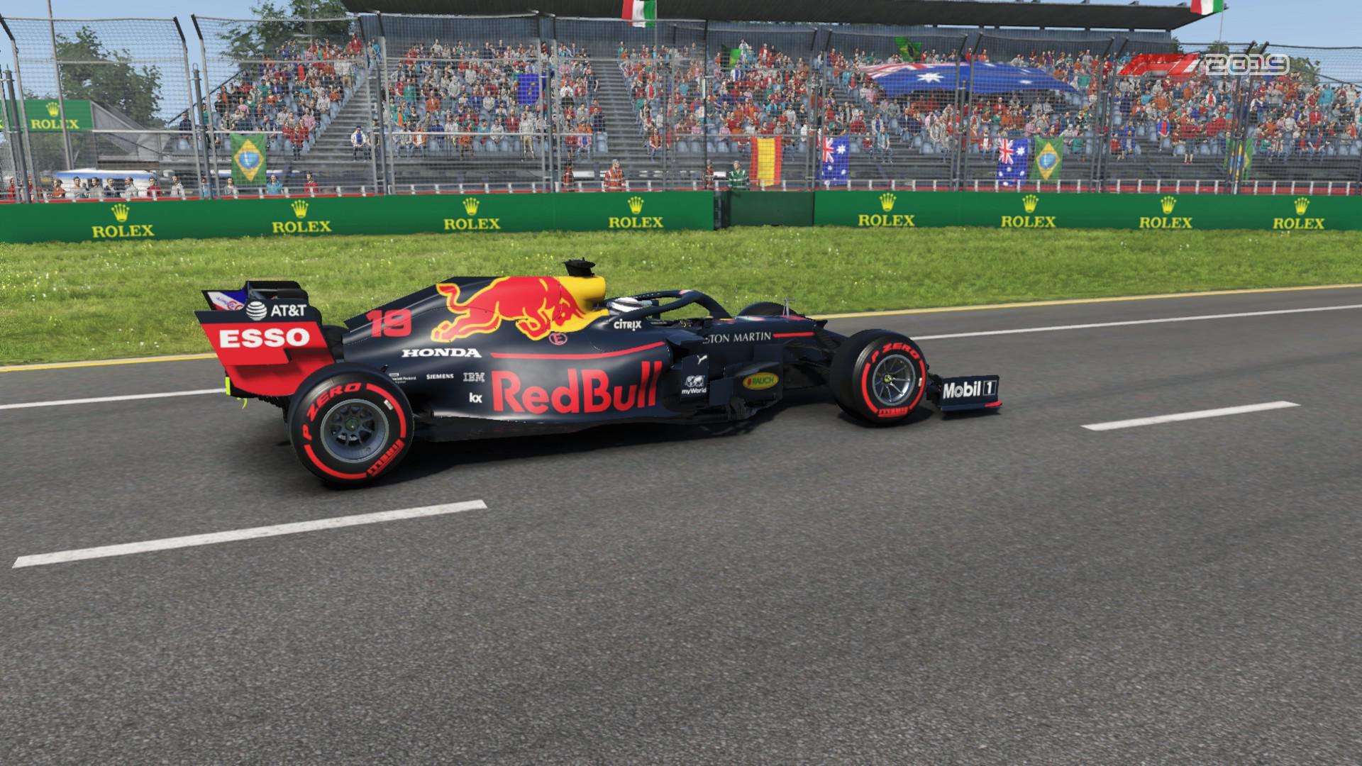
2. Validation: This dataset contains very similar images as in the training set, in the same 10 folders that correspond to the 10 F1 teams.

   Here's a look at a validation image from the Redbull folder.

   

3. labels.txt: A simple txt file that contains the names of the 10 teams in alphabetic order, separated by a newline character.

   1. alfa_romeo

   2. bwt

   3. ferrari

   4. haas

   5. mclaren

   6. mercedes

   7. redbull

   8. renault

   9. toro_rosso

   10. williams

Simply set the paths to the respective folders.

train_dir = '/kaggle/input/f1-cars/f1cars/train' #@param {type: "string"}
val_dir = '/kaggle/input/f1-cars/f1cars/val' #@param {type: "string"}

Convert Dataset Into TensorFlow Dataset

You need to load your data as a tensorflow.data.Dataset to pass it as an input to any Transfer Learning model.

There are many functions in the keras API to achieve this, I used the image_dataset_from_directory function.

IMG_SIZE= 224

train_data = keras.utils.image_dataset_from_directory(
    train_dir,
    labels="inferred", #infer the label of each image as its foldername
    label_mode="categorical", #used for categorical entropy loss
    color_mode="rgb", #3 colour channels
    image_size=(IMG_SIZE, IMG_SIZE), #(224,224)
)

val_data = keras.utils.image_dataset_from_directory(
    val_dir,
    labels="inferred", #infer the label of each image as its foldername
    label_mode="categorical", #used for categorical entropy loss
    color_mode="rgb", #3 colour channels
    image_size=(IMG_SIZE, IMG_SIZE), #(224,224)
    shuffle = False #important line!!
)

#Create a list of labels (team names)
class_names=train_data.class_names

# prefetching the datasets for faster training
train_data=train_data.prefetch(tf.data.AUTOTUNE)
val_data = val_data.prefetch(tf.data.AUTOTUNE)

Visualize The Training Data

You can visualize the training data along with the corresponding labels, just to confirm if a given image is assigned to the right label.

This is one of the many ways to confirm that the data has been loaded correctly.

plt.figure(figsize=(10, 10))
for images, labels in train_ds.take(1):
    for i in range(9):
        ax = plt.subplot(3, 3, i + 1)
        plt.imshow(np.array(images[i]).astype("uint8"))
        pred_class = np.argmax(labels[i])
        plt.title(classes[pred_class])
        plt.axis("off")

Here's the output of the above lines of code:

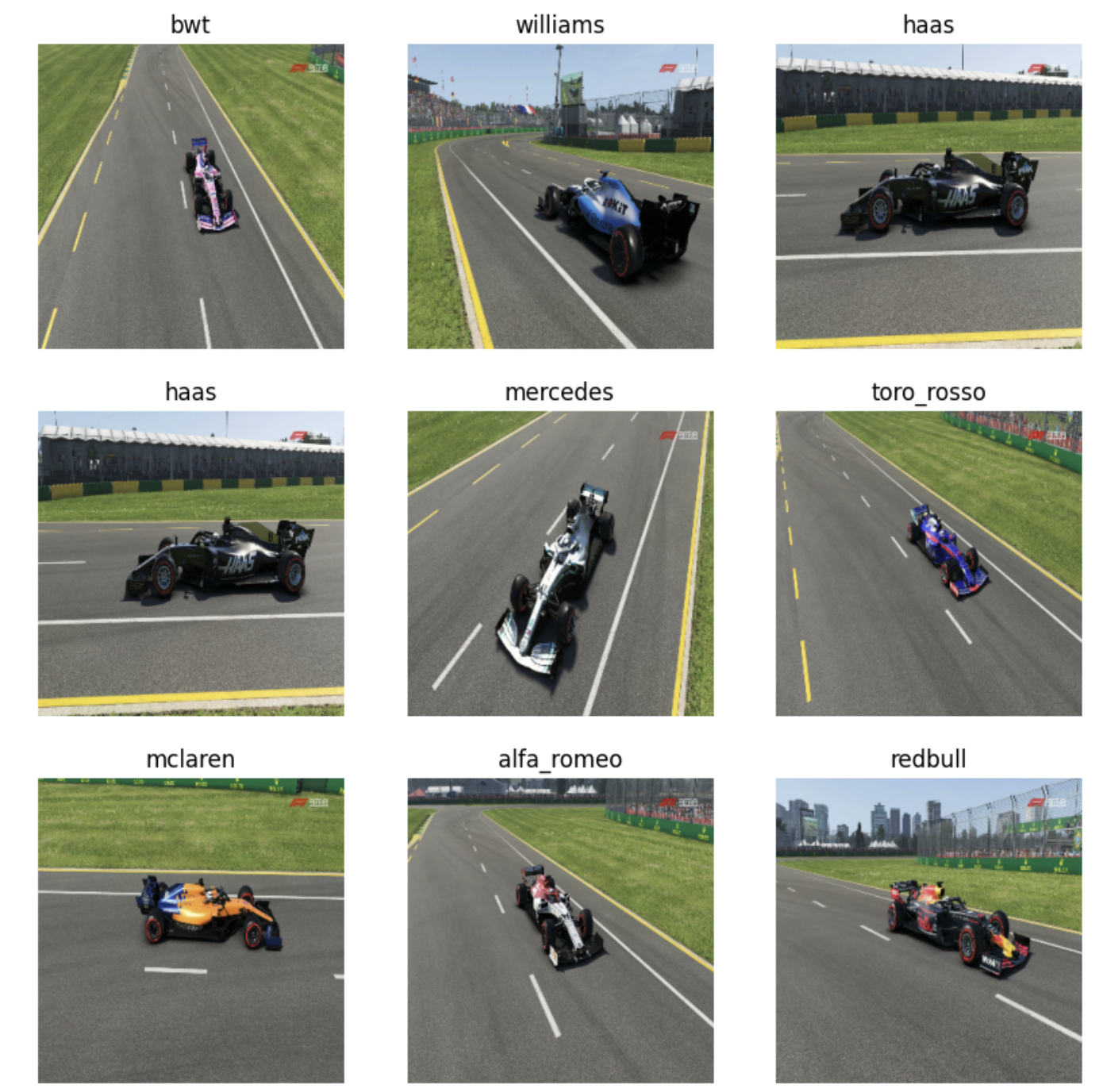
The above plot confirms that the data has been loaded correctly.

Perform Data Augmentation

Data Augmentation is a crucial step to create more data from existing data.

This can be done by randomly rotating, zooming, changing the brightness, changing the contrast of the existing images, and using the newly created images along with current images as training data.

Theoretically, this helps the model generalise better and prevent over-fitting to the training set.

Plus, since we're not training the model from scratch but rather, just using its pre-trained weights, the more data we have, the merrier.

Here, we build a separate Data Augmentation layer that will be used in the Model Building section, to modify the images on the fly, i.e, while training.

data_augmentation = Sequential(
    [
        layers.RandomFlip("horizontal"),
        layers.RandomRotation(0.1),
        layers.RandomZoom(0.1),
        layers.RandomContrast(0.1),
        layers.RandomBrightness(0.1),
    ]
)

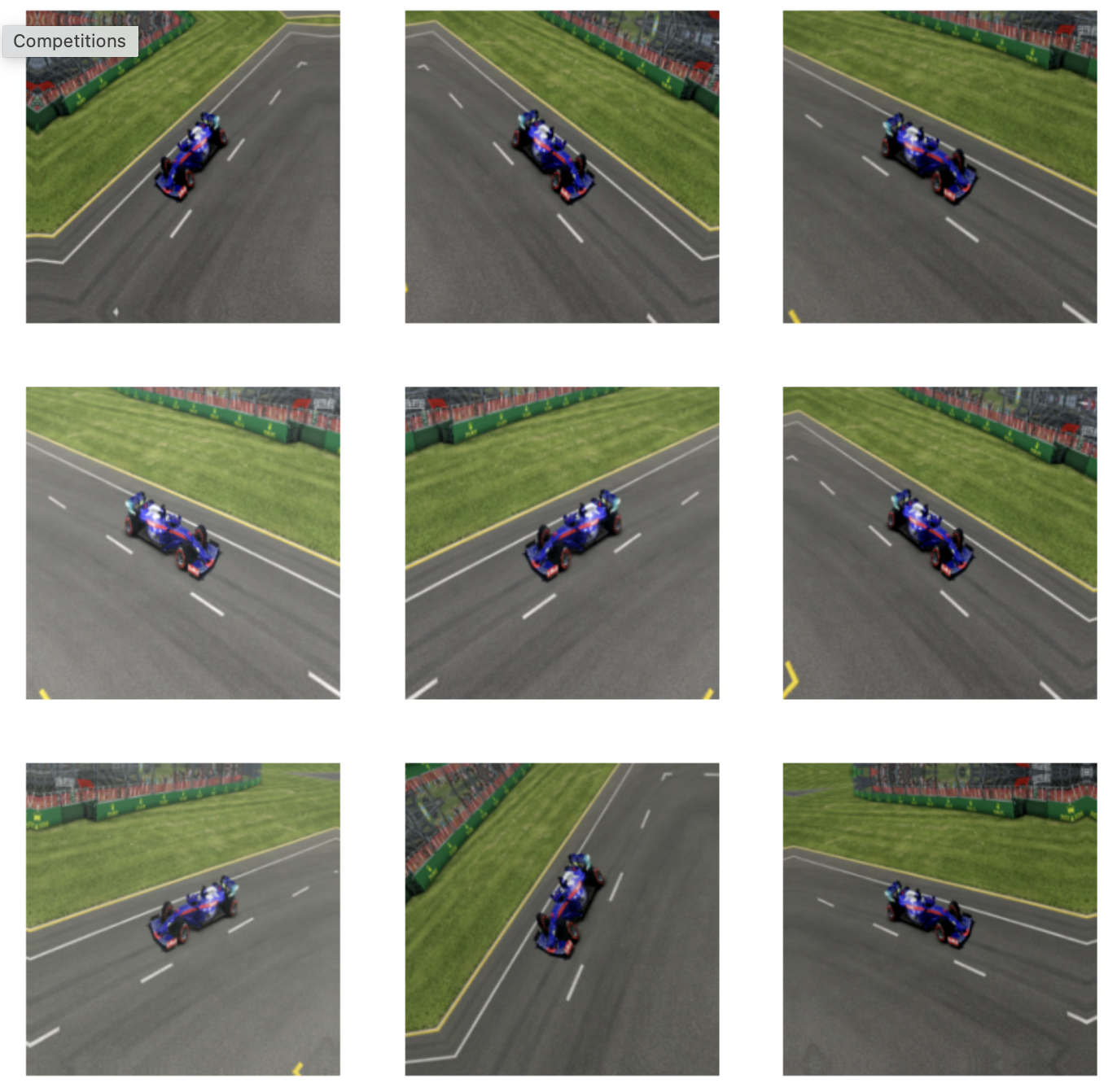
Let's visualize what this data augmentation does to a set of images using the below piece of code.

plt.figure(figsize=(10, 10))
for images, _ in train_ds.take(1):
    for i in range(9):
        augmented_images = data_augmentation(images)
        ax = plt.subplot(3, 3, i + 1)
        plt.imshow(np.array(augmented_images[0]).astype("uint8"))
        plt.axis("off")

Below is the output for the above code.

Perform Transfer Learning

When doing Transfer Learning, we need to get headless models.

For some context, a headless model is the original model without its top prediction layer.

In this classifier, I utilised the EfficientNet-B0 image classification model that had been trained on the ImageNet Dataset.

Why EfficientNetB0?

The reason for choosing EfficientNetB0 can be explained via the graph from the EfficientNet Paper below.

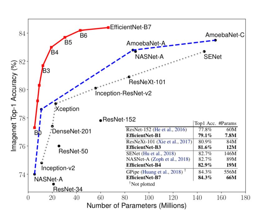
If you look closely towards the bottom left, you can see B0 with the least amount of parameters and still a decent accuracy of ~77% on the ImageNet dataset.

However, it's logical to think - Why not EfficientNet-B7? It clearly has relatively less number of parameters for the highest accuracy among all the models in the graph.

And you know what, I initially went with it.

But, due to lack of availability of strong GPU power, running only 5 epochs took me more than 30 mins!

Hence, B0😊

Build The Model

The base model used in this tutorial is available in the keras applications API.

A useful tip for you: don't import the model from tensorflow hub if you're working locally or on Kaggle, it won't work. That only works on Google Colab.

mixed_precision.set_global_policy('mixed_float16') #faster calculations

#input layer
inputs=layers.Input(shape=(224,224,3),name='input_layer') 

#download model EfficientNet-B0
base_model=keras.applications.efficientnet.EfficientNetB0(include_top=False)
base_model.trainable=False #Freeze Weights of base model

#apply data augmentation on the fly
x = data_augmentation(inputs)

#pass x through the base model 
x=base_model(x,training=False)

#pooling layer
x=layers.GlobalAveragePooling2D(name='Global_Average_Pool_2D')(x) 

#batch norm layer
x = layers.BatchNormalization()(x) 

#dropout layer
top_dropout_rate = 0.2
x = layers.Dropout(top_dropout_rate, name="top_dropout")(x) 

#prediction (dense) layer with number of units = number of classes
num_classes=len(class_names)
outputs=layers.Dense(num_classes,activation='softmax',dtype=tf.float32,name="Output_layer")(x)

#final model
model=keras.Model(inputs,outputs,name="model")

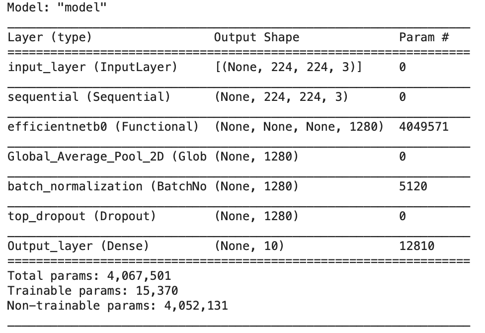
Here's a summary of the model that we built.

You may manually save the initial, pre-trained weights of the model to load them whenever you want as:

model.save_weights('initial_weights.weights.h5')

Create Callback

Simply speaking, callbacks are great.

I would recommend you to learn about them and always use them whenever you're training a model.

They make the learning process efficient and time saving!

This becomes very important when you have limited computational resources at your disposal.

For transfer learning, I created a simple Model Check Point callback that would store the new "best" weights of the model for every epoch if the validation loss improves for the corresponding epoch.

# Get the current working directory
current_dir = os.getcwd()

# Create the "ModelCheckPoints" directory
model_checkpoint_dir = os.path.join(current_dir, 'ModelCheckPoints')
os.makedirs(model_checkpoint_dir, exist_ok=True)

def create_model_check_point_callback(checkpoint_path,monitor='val_loss'):
    """
    Takes the path where to save the best model weights obtained during training.
    """
    model_checkpoint_cb=tf.keras.callbacks.ModelCheckpoint(

        monitor=monitor,
        filepath=checkpoint_path,
        save_best_only=True,
        save_weights_only=True,
        save_freq='epoch',
        verbose=1
    )
    return model_checkpoint_cb

The above code shows that while training the model, after every epoch, if the validation loss decreases, the new model weights will get saved to the provided checkpoint path.

Compile And Fit Model on Training Data

Compile the model with the standard :

1. Categorical entropy loss

2. Adam optimizer with the default learning rate 0.001

3. Accuracy metric

model.compile(
    loss=keras.losses.categorical_crossentropy,
    optimizer=keras.optimizers.Adam(),
    metrics=['accuracy']
)

Fit the model on training data using val_data as validation data with Model Check Point as callback.

ModelCheckPoint_model_cb=create_model_check_point_callback('./ModelCheckPoints/model.weights.h5')
EPOCHS=5
history_of_model=model.fit(
    train_data,
    epochs=EPOCHS,
    steps_per_epoch=len(train_data), #batch size
    validation_data=val_data,
    validation_steps=len(val_data),
    callbacks=[ModelCheckPoint_model_cb]
)

Perform Fine-Tuning

The first step for fine tuning is unfreezing some of the top layers.

This means that the parameters in the unfreezed layers will be trainable, i.e., this will help the model learn the training data well and generalize better on the validation data.

Unfreeze Layers

The below code is inspired from an image classification tutorial by Keras. Click Here to view it.

Here, the top 20 layers of EfficientNet-B0 are being unfreezed.

def unfreeze_model(model):
    # We unfreeze the top 20 layers while leaving BatchNorm layers frozen
    for layer in model.layers[-20:]:
        if not isinstance(layer, layers.BatchNormalization):
            layer.trainable = True

    #compile the model
    optimizer = keras.optimizers.Adam(learning_rate=1e-5)
    model.compile(
        optimizer=optimizer, loss="categorical_crossentropy", metrics=["accuracy"]
    )


unfreeze_model(model)

Create More Callbacks

With Fine-Tuning, we will train the model for much longer than 5 epochs.

Sometimes, the validation loss plateaus (doesn't decrease) or, the model reaches peak training accuracy such that we don't need to train it anymore.

Hence, apart from the Model Check Point callback (storing the best weights of the model), two more callbacks are implemented:

1. Early Stopping: Stop training if the training accuracy reaches 100% before all epochs are finished. Hence, saving a lot of time.

2. Reduce Learning Rate On Plateau: Reduce the learning rate by a factor of 0.2 if the validation loss doesn't decrease for 3 epochs consecutively.

#Utilising the Model Check Point Callback
ModelCheckPoint_model_cb=create_model_check_point_callback('./ModelCheckPoints/model_2.weights.h5')
# defining early stopping callback
early_stopping_cb=tf.keras.callbacks.EarlyStopping(patience=5,restore_best_weights=True,verbose=1)
# defining reduce learning rate on plateau callback
reduce_lr_cb=tf.keras.callbacks.ReduceLROnPlateau(factor=0.2,patience=3,min_delta=1e-3,min_lr=1e-7,verbose=1)

Continue Fitting Model On Training Data

The model was trained for 25 more epochs post transfer learning through fine tuning.

fine_tune_epoch=EPOCHS+25
history_of_model_2=model.fit(
    train_data,
    epochs=fine_tune_epoch,
    initial_epoch=EPOCHS-1,
    steps_per_epoch=len(train_data),
    validation_data=val_data,
    validation_steps=len(val_data),
    callbacks=[ModelCheckPoint_model_cb,early_stopping_cb,reduce_lr_cb]
)

Results

Here are the results that were obtained.

Transfer Learning

Upon running the initial model (without fine-tuning) for 5 epochs, the categorical cross entropy loss and the accuracy on the validation data were as follows.

68% accuracy on the validation set indicated that the Transfer Learning model wasn't able to generalise well to the data that it hadn't seen.

A greater insight was offered by plotting the training and validation losses and accuracies over the epochs, as shown by the graphs below.

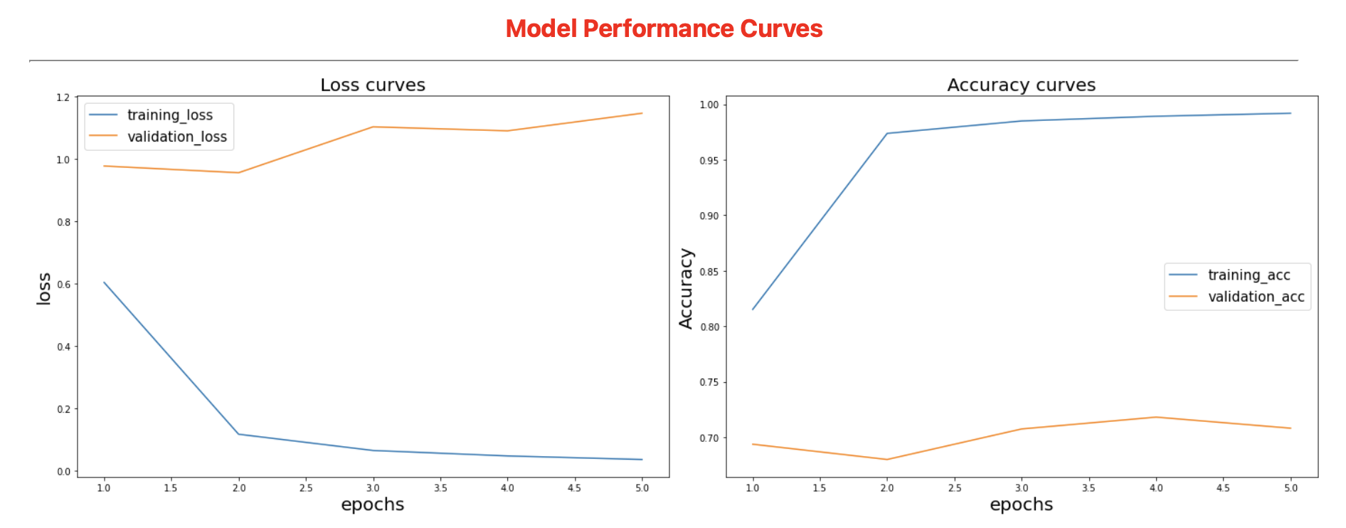
This shows that the model was clearly overfitting on the training data, with training accuracies sky high and training losses extremely low, while validation accuracies were very low and validation losses were higher.

Fine-Tuning

After Fine-tuning the model and reducing the learning rate by 100 times, the results obtained on the validation dataset are shown below.

An increase of ~30% from the transfer learning model was noticed in the accuracy on validation set. The loss went down by ~52% as well after fine tuning!

Although the results for fine-tuning were much better than transfer learning, a different angle to the story is shown by the graphs below

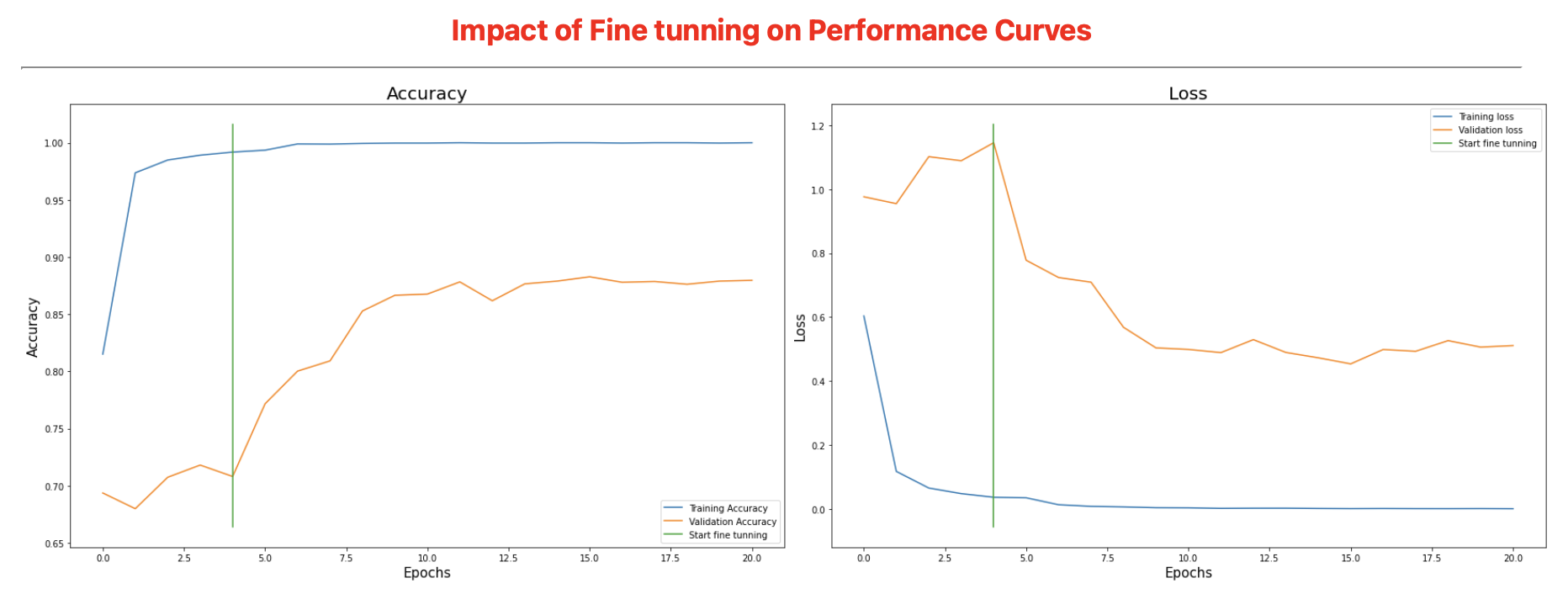
To the left of the green line are the results of Transfer Learning, and to its right are the results for Fine-Tuning.

Clearly, the model was still overfitting the training data, with training accuracies reaching 100% and losses reaching to 10^-4!!

Confusion Matrix (HeatMap)

To better grasp the scale of overfitting and understand where the model is going wrong and where it is going right, a confusion matrix was plotted.

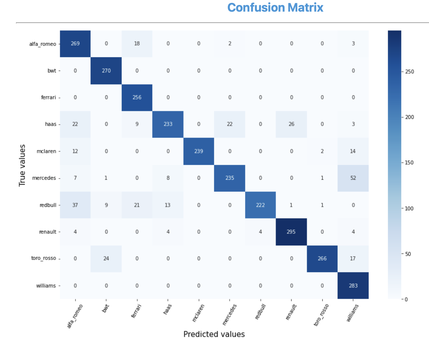
The above confusion matrix clearly shows that the model was able to get most of the cars right.

However, there were few pairs of cars that it had some difficulty in classifying:

1. Mercedes & Williams (52 mislabelled)

2. Redbull & Alfa Romeo (37 mislabelled)

3. Haas & Renault (26 mislabelled)

Conclusion

Overall, an accuracy of ~89% is still appreciable, and this approach clearly showed how fine tuning a model to a particular dataset can make a difference w.r.t transfer learning.

I would love to hear your suggestions on improving this accuracy in the comments below!

Some Important Lessons Learnt

However simple this task might have been, it still taught me a lot about the minute details of solving a Machine Learning problem.

Some of them being:

1. CPU vs GPU in regards to data augmentation

2. Saving and loading model weights manually

3. Efficient use of callbacks

4. Avoiding Batch Norm Layer while unfreezing the model to maintain accuracy

5. Importance of Confusion Matrix in realising model performance

I believe that there is no course that can teach such tiny details about the implementation of a ML task.

These things can only be learnt by doing and getting your hands dirty (metaphorically).

I've noticed that my level of comfort with tools like Tensorflow, Keras, and python in general is increasing with every side project that I do.

And I hope that you've learnt something valuable from this blog as well.

Congratulations on making it to the end of this blog!

Want to receive my blogs directly in your inbox? Enter your email ID below to join my newsletter!