Hey there, fellow data enthusiasts!

This week, we will explore the intricacies of Spark Internals, from DataFrame Writer API and various write modes to advanced partitioning and bucketing techniques. We will discover how to optimize query performance, manage parallelism, and efficiently allocate resources in Spark.

Dataframe Writer API

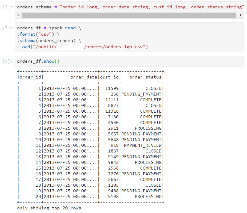
Consider the following orders dataset.

The path to the folder where the results need to be written, must be specified while writing the results using the dataframe writer.

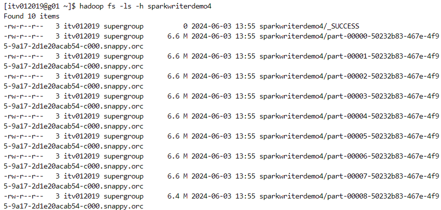
The data looks like this after the write operation. Note that we are using the CSV file format.

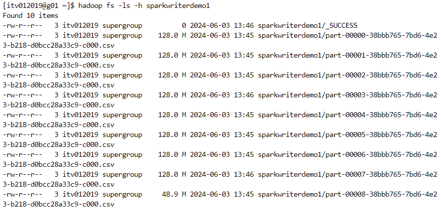
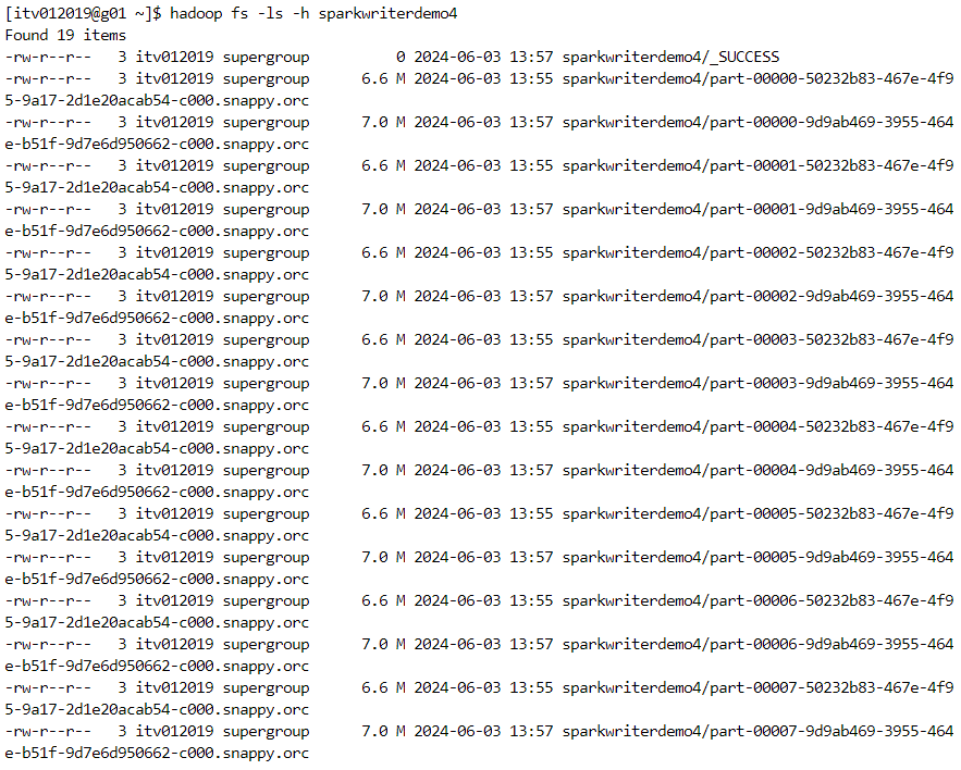
Since we have specified the mode as overwrite, if we perform the operation again, the data will get overwritten.

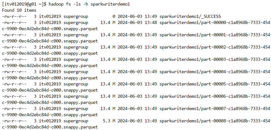
We can use various other file formats while writing to the dataframe.

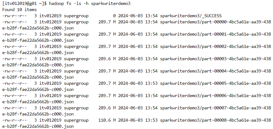
json: a bulky file format that has to embed the column names for each record, thus consuming large amounts of space.

orc: a good file format in terms of optimization.

Other file formats that can be considered are:

parquet: the most optimized and compatible file format for spark.
avro: an external data source that requires the setting up of specific cluster configurations.

Write modes in Spark

overwrite: if the folder where the results need to be written exists already on the disk, then it will be overwritten.
ignore: if the folder already exists at the specified path, the writing files will be ignored.
errorIfExists: if the folder already exists, then the write operation would invoke an error.
append: if the folder already exists at the path mentioned, the new files will be appended to the existing folder.

Partitioning

Partitioning is the process of structuring the data in an efficient way in the underlying file system, such that only a subset of data gets scanned when a query is fired instead of the entire data, thus resulting in performance gains.
Consider the following example dataset 'orders', and the query.

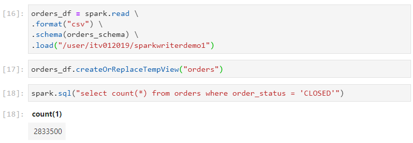
The query execution time will be high because all the files have to be scanned for processing the query.

In order to optimize the query performance, the data need to be partitioned such that only a subset of data gets scanned.

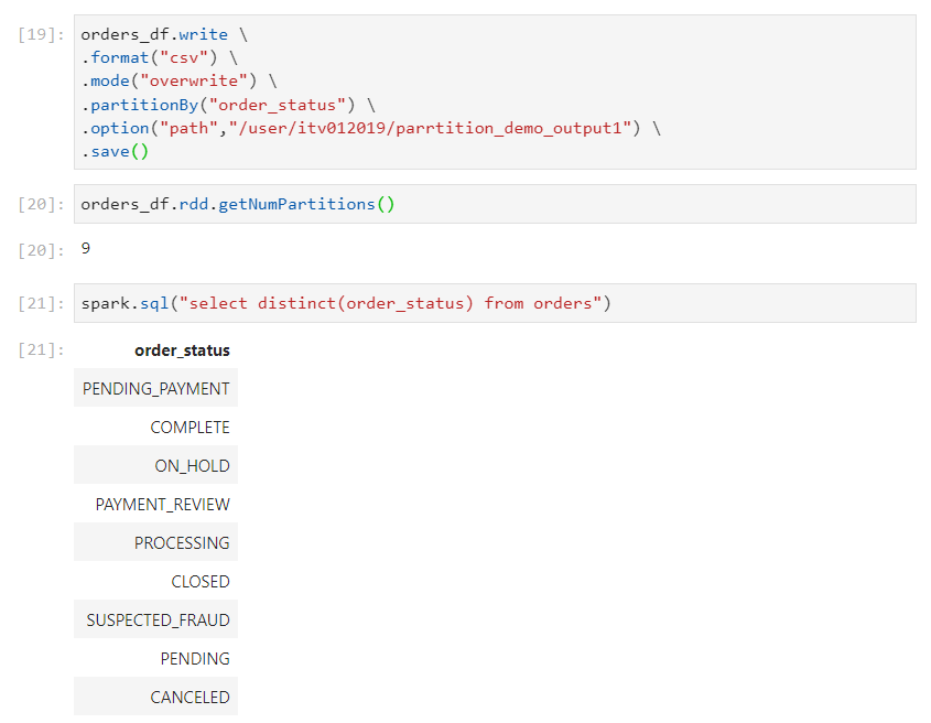
For the above write operation, since we are using the order_status column for partitioning, folders will be created on the basis of distinct order status'.
Ideally, partitionBy should be applied on the column which has less number of distinct values, as we are doing in this case.

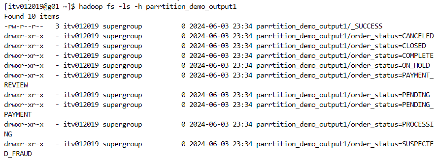
Since the number of partitions is 9, 9 files will be created within each order_status folder.

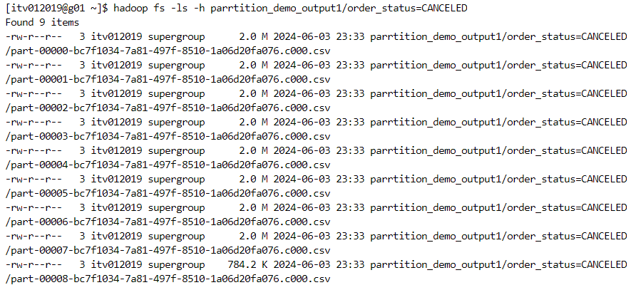
Now, if we perform the same query on the partitioned data, only the necessary partitions will be scanned and the rest of the partitions will be skipped. This process is known as partition pruning.

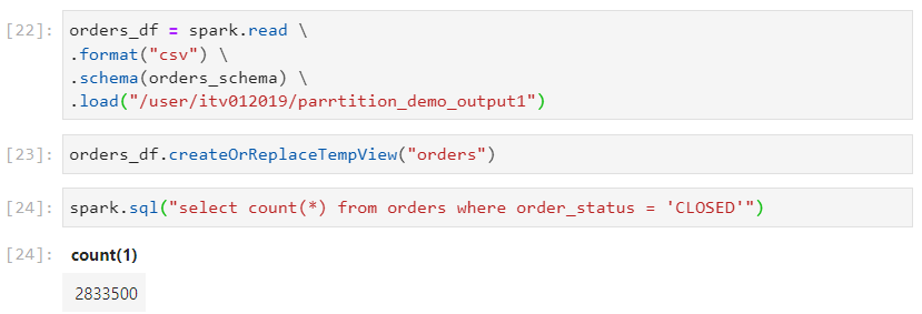
Interestingly, only 9 files inside the particular order_status get scanned.

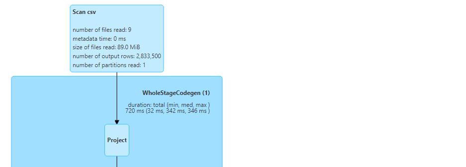
Similarly for other values of order_status.

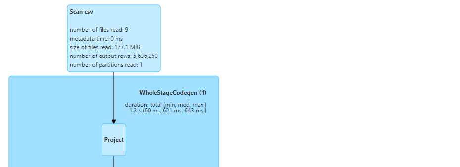
Note that if filtering is applied on any non-partitioned column, we would not get any performance gains.

All the files get read here.

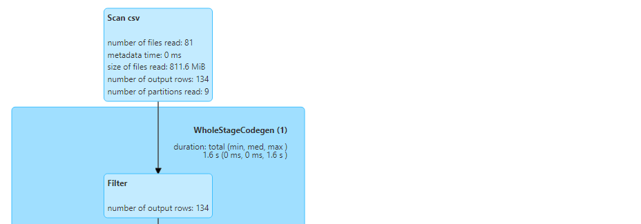
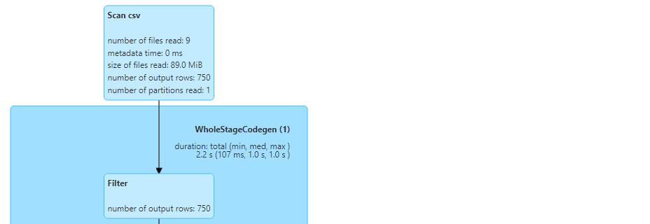
However, if the partitioned column is included first and thereafter the next column is filtered upon, performance benefits get achieved.

Now, consider the following customers dataset. We want to apply partitioning on both customer_state and customer_city.

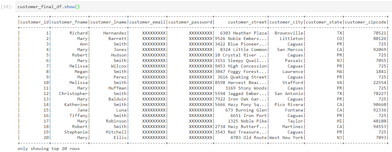
Partitioning can be applied simultaneously on more than one column, by specifying the list of columns in the partitionBy clause.

Now, the top-level folders get created for each state.

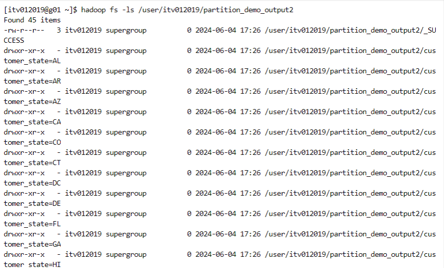
Inside each top-level state folder there are sub-levels of city folders. Inside each city folder, there are files containing the actual data.

Let us consider the case where we perform all of the above operation i.e. two levels of folders and store the data in parquet file format.

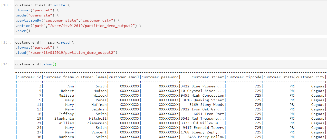
If we don't incorporate the partitioning benefits, we get the following query execution performance.

However, if we filter on the basis of partitioned columns, the query performance benefits are immense.

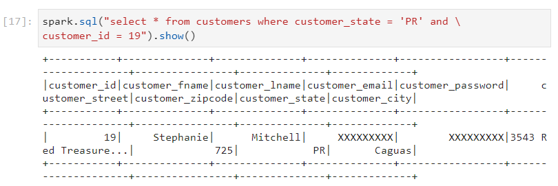
The number of files read reduce drastically.

If we perform filtering upon both the partitioned columns, only one file gets read.

Bucketing

When the number of distinct values are large, then bucketing is a better choice over partitioning. In bucketing, the number of buckets and the bucketing column have to be specified upfront as parameters to the bucketBy clause.

Every partition will have files equal to the number of buckets mentioned while creating the dataframe.

For checking the performance, we first run a query on a non-bucketed column.

Now, upon running the query on a bucketed column of the bucketed table, we observe significant rise in the performance, in terms of the number of output rows and scan time.

It is interesting to note that a combination of partitioning followed by bucketing is possible, whereby two levels of optimized filtering can be achieved.

Spark Internals

For checking the default parallelism in Spark:

By default, dynamic allocation of executors is enabled for the cluster.

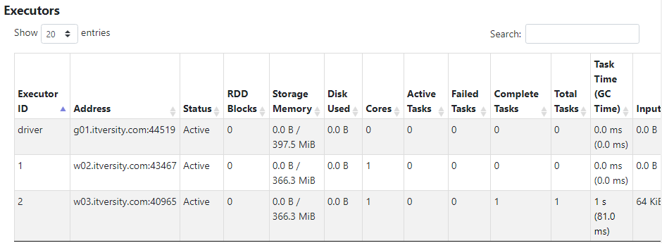
Default parallelism is 2 because there are 2 executors available with 1 core and 1 GB RAM each.
Parallelism depends upon the amount of resources that are allocated. If an application holds 16 cores then the parallelism will be 16. In our case, there are 2 cores, therefore the parallelism is 2.

How distinct() works?

Considering the orders dataset of ~1.1 GB, there would be 9 partitions created for this dataset based on the default partition-size of 128 MB.
Now, consider the following distinct command. There are 9 distinct order status'.

Initially, 9 partitions get created, each partition sends the local results to a common node through shuffling, where the final aggregation gets carried out.

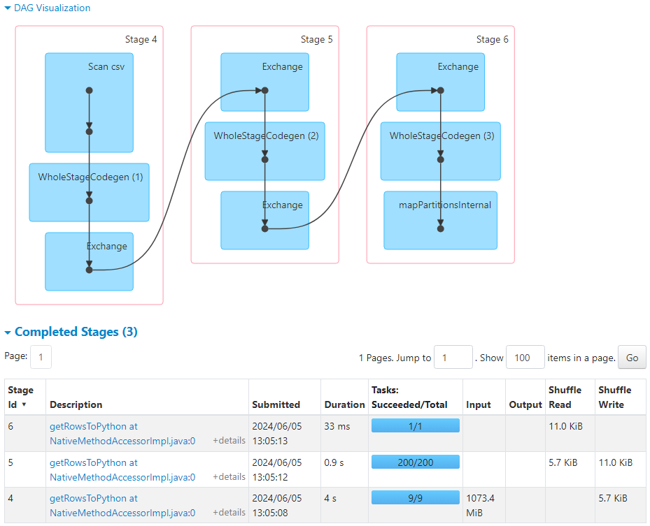
9 tasks get launched to load the dataframe. Since dynamic allocation is enabled, executors get allocated to the tasks as per their availability.

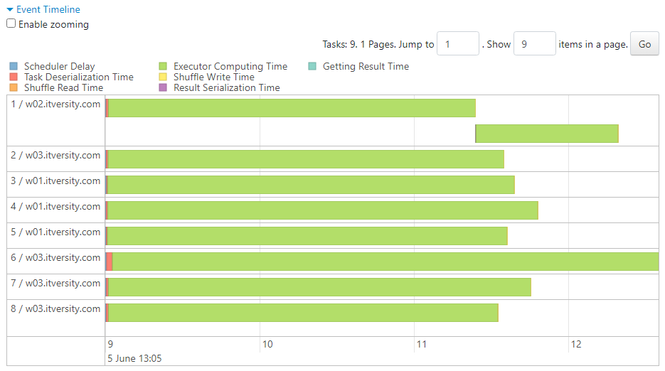
In case of queries where shuffling is not involved:

Executors become available for the upcoming task as soon as they complete the previous task at hand.

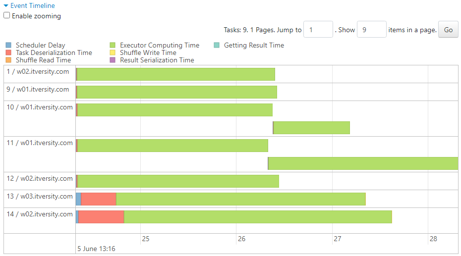
Upon executing the same query twice, more executors get allocated, thus increasing the default parallelism from 2 to 8.

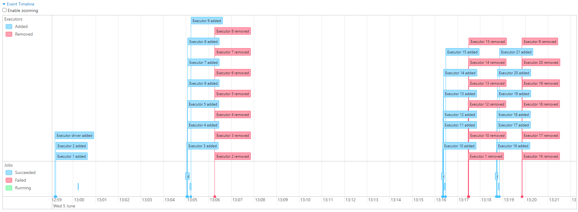
Disabling dynamic executor allocation

We can turn off the dynamic allocation and request a static amount of resources as well.

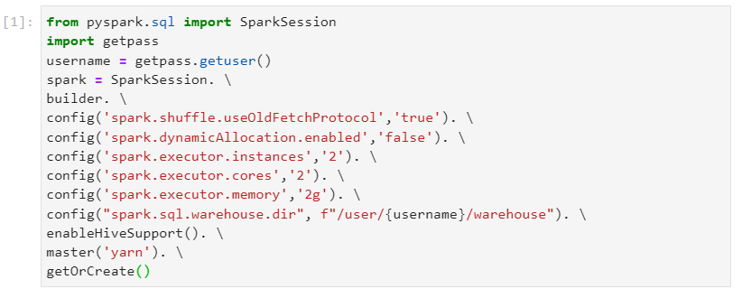
As we can see, the required number of cores get allocated, as per specifications.

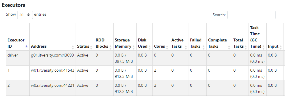
Since there are 4 cores available, default parallelism will also be 4.

Now, upon execution of the following query,

The 9 tasks get executed as per the parallelism of 4, where each executor becomes available dynamically.

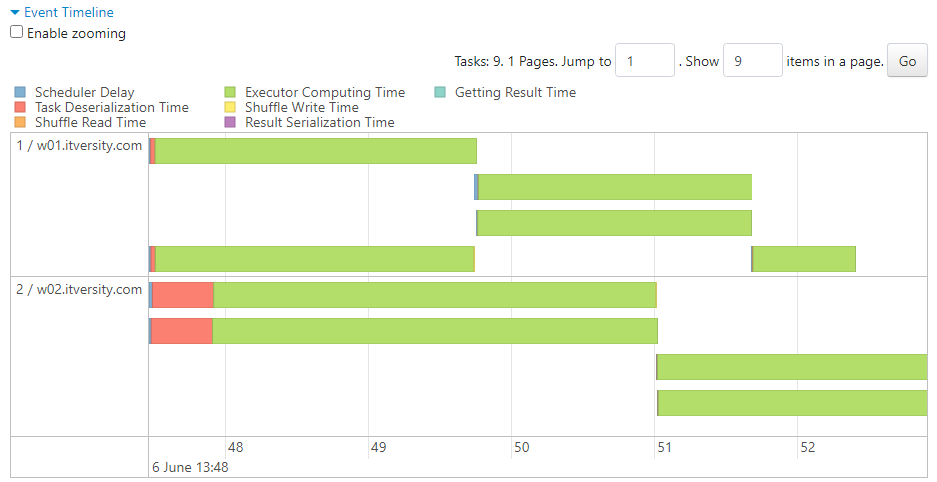
The disadvantage of static resource allocation is that the resources can go idle when there are less tasks to be executed. To overcome this, spark-submit can be used to execute the jobs on cluster.

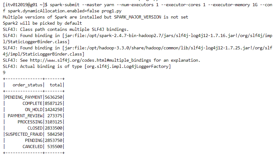
Spark submit

It is a utility to package the code and deploy it on the cluster. Let us say, the code is written in prog1.py file.

Initial number of partitions in a dataframe

Number of partitions play an important role in determining the level of parallelism that can be achieved.
Initial number of partitions depend primarily upon two configurations:
- Default parallelism - number of CPU cores in the cluster
- Default partition size
If the partition size is large, it can lead to out-of-memory error because data may not fit into the execution memory of the machine.
Number of initial partitions is determined by the partition size, and recommended partition size is 128 MB.

Calculating the initial number of partitions for a single non-splittable file

Partition size and default parallelism are as follows.

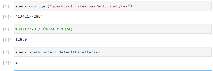
Usage of compression techniques like Snappy or GZip with csv file format will lead to non-splittable files.

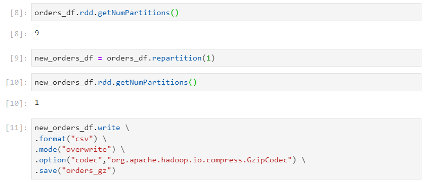
In case of a non splittable file, only one partition will get created.

Calculating the initial number of partitions for multiple file

In case of multiple files, if the partition size is less, 2 or more files will be combined into one partition to approximately make up to the default partition size of 128 MB.

Following are the splittable files, due to the codec/snappy compression techniques.

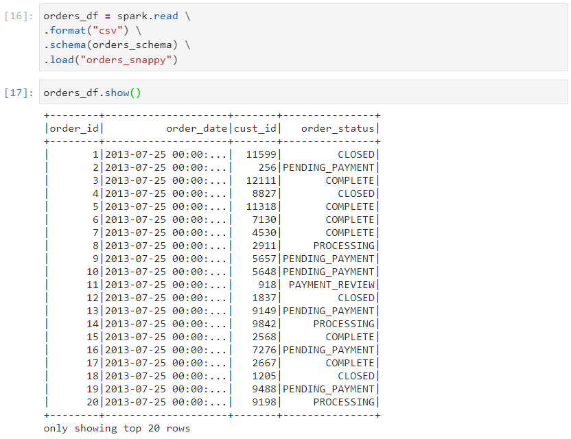
If there are 20 multiple files of 53 MG each, then 2 files will be combined together to reach a default partition size of 128 MB.

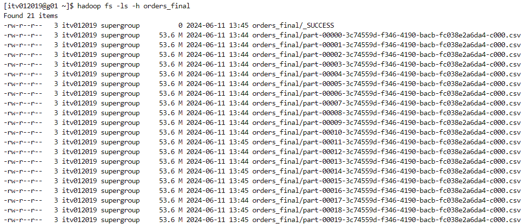
Therefore, 10 partitions would be created in this case.

Conclusion

Understanding Spark internals is crucial for maximizing the efficiency and performance of your data processing tasks. By mastering DataFrame Writer API, partitioning, bucketing, and resource allocation, you can significantly enhance the speed and reliability of your Spark applications. Keep experimenting with different configurations and optimizations to find what best suits your data needs.

Stay tuned for more deep dives into the world of data engineering!

Week 6: Spark Internals Demystified 🔮