Chapter 2 - Hands on with the World of Multimodality
 Hrishikesh Yadav
Why is there a need for multimodality?
The need for sophisticated technologies that can comprehend and process the diversity of information that exists in today's digital age—text, images, audio, and video—is critical. The key to overcoming this difficulty is multimodality, or a system's capacity to handle several data types at once. Industries ranging from healthcare to gaming are increasingly recognizing the importance of multimodal solutions.
Multimodal models offer a number of benefits, including the capacity to analyze data from several sources at once, which broadens the picture and facilitates greater context and self-learning. Due to the shortcomings of single-data-type models, this increased comprehension results in increased accuracy, better decision-making, and the capacity to take on tasks that were previously difficult. To achieve more accurate and contextually rich results, multimodal models can take advantage of both the complexities of visual content and the subtleties of natural language, which traditional AI models might find difficult to handle separately.
What all Data Modalities are there
Text
Audio
Video
Image
Depth (3D)
Thermal (Infrared Radiation)
Internal Measurement Unit
How various modalities are configured - Contrastive Learning
Contrastive learning performs exceptionally well in situations where labeled data is either nonexistent or very scarce. Since the model is trained to identify patterns without explicit labels, this makes it especially useful for self-supervised learning. Contrastive learning can be used in supervised situations where labels are available as well, providing a useful alternative to more conventional approaches. It is not, however, restricted to unlabeled data.
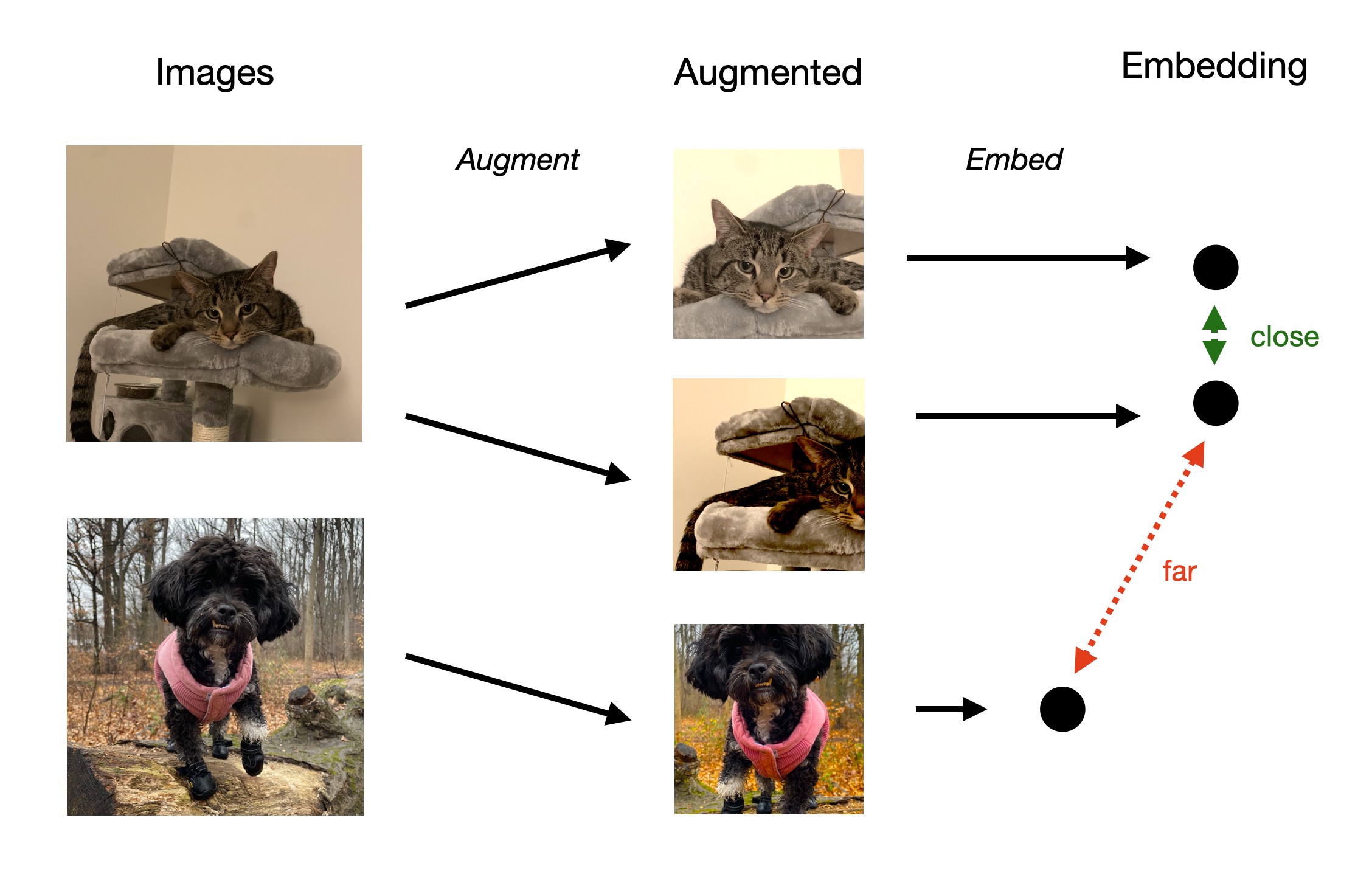
The ideas of anchors, positives, and negatives form the basis of contrastive learning. Consider an anchor as a point of reference—a specific piece of information that you are concentrating on. Positives and the anchor are comparable in that they have similar traits or fall into the same group. Negatives act as contrasts to the anchor and are clearly different from the anchor. The objective is to move negatives farther away from the anchor and positives closer to it in a multidimensional space called the embedding space.

For example, a picture of a cat could serve as an anchor. Negative images could be something unrelated to cats, like a dog, but positive images might be of other cats, maybe in various colors or positions. The learning algorithm's job is to modify these images' embedding space representation so that, while photos of dop or unrelated images stay far apart, photographs of cats cluster together (positively).

One Database for Multimodal Data
Storing the multimodal data into the embedding form into the one database helps to provide more personalization and flexibility to the user and opens up new path for the usecases.
This helps to build the Any to Any Search Applications capabilities. It focuses on showcasing how any of the modalities that the multimodal model understands and embeds may be sent in as a query and can return objects of any modality that share conceptual similarities. We will be discussing on the Hands-on way to build any to any search application in the upcoming blog of the series.

Let's Play with Contrasive Learning
Importing the necessary libraries -
import numpy as np
import pandas as pd
import matplotlib.pyplot as plt
from tqdm.notebook import tqdm
from sklearn.decomposition import PCA
Some, Libraries for the plotting
import umap
import umap.plot
import plotly.graph_objs as go
import plotly.io as pio
Importing, more modules which will be needed for the construction of model
import torch
from torch import nn, optim
from torch.utils.data import DataLoader
from torchvision import transforms
Now, we will setup the MNIST script to transform the dataset
import pandas as pd
from torch.utils.data import Dataset
import numpy as np
from tqdm import tqdm

class MNISTDataset(Dataset):
    def __init__(self, data_df: pd.DataFrame, transform=None, is_test=False):
        # For the intiaition of the function
        super(MNISTDataset, self).__init__()
        dataset = []
        labels_positive = {}
        labels_negative = {}
        if is_test == False:
            for i in list(data_df.label.unique()):
                labels_positive[i] = data_df[data_df.label == i].to_numpy()
            # for each label create a set of image of various label
            for i in list(data_df.label.unique()):
                labels_negative[i] = data_df[data_df.label != i].to_numpy()

        for i, row in tqdm(data_df.iterrows(), total=len(data_df)):
            data = row.to_numpy()

            if is_test:
                label = -1
                first = data.reshape(28, 28)
                second = -1
                dis = -1
            else:
                # label and image of the index for each row in df
                label = data[0]
                first = data[1:].reshape(28, 28)
                # probability of same label image == 0.5
                if np.random.randint(0, 2) == 0:
                    # randomly select same label image
                    second = labels_positive[label][
                        np.random.randint(0, len(labels_positive[label]))
                    ]
                else:
                    # randomly select different label
                    second = labels_negative[label][
                        np.random.randint(0, len(labels_negative[label]))
                    ]
                # cosine is 1 for same and 0 for different label
                dis = 1.0 if second[0] == label else 0.0
                second = second[1:].reshape(28, 28)

            # apply transform on both images
            if transform is not None:
                first = transform(first.astype(np.float32))
                if second is not -1:
                    second = transform(second.astype(np.float32))
            # this random list is created once and used in every epoch
            dataset.append((first, second, dis, label))

        self.dataset = dataset
        self.transform = transform
        self.is_test = is_test

    def __len__(self):
        return len(self.dataset)

    def __getitem__(self, i):
        return self.dataset[i]
You can download the training and the testing dataset of the MNIST from here -
df = pd.read_csv('digit/train.csv')
val_count = 1000
default_transform = transforms.Compose([
    transforms.ToPILImage(),
    transforms.ToTensor(),
    transforms.Normalize(0.5, 0.5)
])

#Setting up the training and the validation set
dataset = MNISTDataset(df.iloc[:-val_count], default_transform)
val_dataset = MNISTDataset(df.iloc[-val_count:], default_transform)
Now, Setting up the dataloader
trainLoader = DataLoader(
    dataset,
    batch_size=16,
    shuffle=True,
    pin_memory=True,
    num_workers=2,
    prefetch_factor=100
)

valLoader = DataLoader(val_dataset,
    batch_size=64,
    shuffle=True,
    pin_memory=True,
    num_workers=2,
    prefetch_factor=100
)
The training loader uses a smaller batch size (16) compared to the validation loader (64). This is common because training often benefits from more frequent updates, while validation can process larger batches at once for efficiency.
Both use 2 worker processes (num_workers=2) for parallel data loading, which can speed up the data pipeline. The prefetch_factor=100 is quite high, which means a lot of data is being preloaded. This can be beneficial if you have enough memory, but you might want to adjust this based on your system's capabilities.
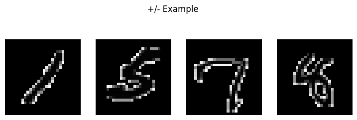
Let's visualize and then observe the anchor and the respective +/- example
import matplotlib.pyplot as plt
import numpy as np

def show_images(images, title='', num_display=4):
    fig, axes = plt.subplots(1, num_display, figsize=(12, 3))
    fig.suptitle(title, fontsize=16)

    for i, ax in enumerate(axes):
        img = np.squeeze(images[i])
        ax.imshow(img, cmap='gray')
        ax.axis('off')

    plt.tight_layout()
    plt.show()

iterator = iter(trainLoader)
anchor_images, contrastive_images, distances, labels = next(iterator)

# Convert to numpy and move to CPU if necessary
anchor_images = anchor_images.cpu().numpy()
contrastive_images = contrastive_images.cpu().numpy()
labels = labels.cpu().numpy()

# Display images
show_images(anchor_images, title='Anchor Images')
show_images(contrastive_images, title='+/- Examples')
Result for the previous snippet -


+/- Examples are the contrasive images.

Let's Build the Neural Network
class Network(nn.Module):
    def __init__(self):
        super(Network, self).__init__()
        self.conv1 = nn.Sequential(
            nn.Conv2d(1, 32, 5),
            nn.BatchNorm2d(32),
            nn.ReLU(inplace=True),
            nn.MaxPool2d((2, 2), stride=2),
            nn.Dropout(0.3)
        )
        self.conv2 = nn.Sequential(
            nn.Conv2d(32, 64, 5),
            nn.BatchNorm2d(64),
            nn.ReLU(inplace=True),
            nn.MaxPool2d((2, 2), stride=2),
            nn.Dropout(0.3)
        )
        self.linear1 = nn.Sequential(
            nn.Linear(64 * 4 * 4, 512),
            nn.ReLU(inplace=True),
            nn.Dropout(0.3),
            nn.Linear(512, 64),
        )

    def forward(self, x):
        x = self.conv1(x)
        x = self.conv2(x)
        x = x.view(x.size(0), -1)
        x = self.linear1(x)
        return x
The network consists of two convolutional layers followed by a fully connected layer.
Conv1 - 1 input channel → 32 output channels, 5x5 kernel
Conv2 - 32 input channels → 64 output channels, 5x5 kernel
Input - 64x4x4 = 1024 features
Hidden layer - 512 neurons with ReLU activation and Dropout Output - 64 dimensional embedding ReLU (Rectified Linear Unit) is used throughout the network inplace=True is used for memory efficiency.
Thus, 64 dimensional embedding is suitable for tasks like contrastive learning or similarity-based comparisons.
class ContrastiveLoss(nn.Module):
    def __init__(self):
        super(ContrastiveLoss, self).__init__()
        self.similarity = nn.CosineSimilarity(dim=-1, eps=1e-7)

    def forward(self, anchor, contrastive, distance):
        score = self.similarity(anchor, contrastive)
        return nn.MSELoss()(score, distance)
The cosine similarity is used to measure the similarity between anchor and contrastive embeddings which is a custom function. Cosine similarity is scale invariant and measures the angle between vectors which helps to distant as per the +/- for the related and unrelated characteristic of the image respectively. Mean Squared Error (MSE) is used to compare the computed similarity with the target distance. The loss encourages similar pairs to have high cosine similarity (close to 1) and dissimilar pairs to have low similarity (close to 0).
optimizer = optim.Adam(net.parameters(), lr=0.001)
loss_function = ContrastiveLoss()
scheduler = optim.lr_scheduler.StepLR(optimizer, step_size=7, gamma=0.4)
The purpose of the above function is to gradually reduce the learning rate during training. It also works on improving the convergence. For the first 7 epochs, the initial learning rate is used. Then, after 7 epochs, the learning rate becomes 30% of it's previous value. The pattern continues every 7 epochs. The advantage of the process is that it helps for the precise optimization. The step size and gamma values may be changed or tuned as per the specific dataset used, so trail and test is the only option.
def model(epoch_count=100):
    net = Network().to(device)
    optimizer = torch.optim.Adam(net.parameters(), lr=1e-3)
    scheduler = torch.optim.lr_scheduler.StepLR(optimizer, step_size=10, gamma=0.1)

    lrs = []
    losses = []
    best_loss = float('inf')
    best_model = None

    for epoch in range(epoch_count):
        net.train()
        epoch_loss = 0
        batches = 0

        print(f'Epoch {epoch+1}/{epoch_count}')
        lrs.append(optimizer.param_groups[0]['lr'])
        print(f'Learning rate: {lrs[-1]:.6f}')

        for anchor, contrastive, distance, _ in tqdm(trainLoader, desc="Training"):
            batches += 1
            optimizer.zero_grad()

            anchor_out = net(anchor.to(device))
            contrastive_out = net(contrastive.to(device))
            distance = distance.to(torch.float32).to(device)

            loss = loss_function(anchor_out, contrastive_out, distance)
            epoch_loss += loss.item()

            loss.backward()
            optimizer.step()

        avg_loss = epoch_loss / batches
        losses.append(avg_loss)
        scheduler.step()

        print(f'Epoch loss: {avg_loss:.4f}')

        # Save the best model
        if avg_loss < best_loss:
            best_loss = avg_loss
            best_model = net.state_dict()
            print(f'New best model saved with loss: {best_loss:.4f}')

        # Save a checkpoint every 10 epochs
        if (epoch + 1) % 10 == 0:
            checkpoint_path = os.path.join(checkpoint_dir, f'model_epoch_{epoch+1}.pt')
            torch.save(net.state_dict(), checkpoint_path)
            print(f'Checkpoint saved at epoch {epoch+1}')

    # Save the best model at the end of training
    best_model_path = os.path.join(checkpoint_dir, 'best_model.pt')
    torch.save(best_model, best_model_path)
    print(f'Best model saved with loss: {best_loss:.4f}')

    return {
        "net": net,
        "losses": losses,
        "best_loss": best_loss
    }
The model() initializes a network, optimizer, and learning rate scheduler. The function runs for a 100 number of epochs, processing batches of data. In each epoch, it computes losses using anchor and contrastive samples, performs backpropagation, and updates the model. It tracks and saves the best performing model based on the lowest average loss. The function saves checkpoints every 10 epochs and the best model at the end of training. It returns the trained network, loss history, and best loss achieved.
import os

# Directory to save the checkpoints
checkpoint_dir = 'checkpoints/'

# Ensure directory exists
if not os.path.exists(checkpoint_dir):
    os.makedirs(checkpoint_dir)

# To call the model() function and start the training
training_result = model()
model = training_result["net"]

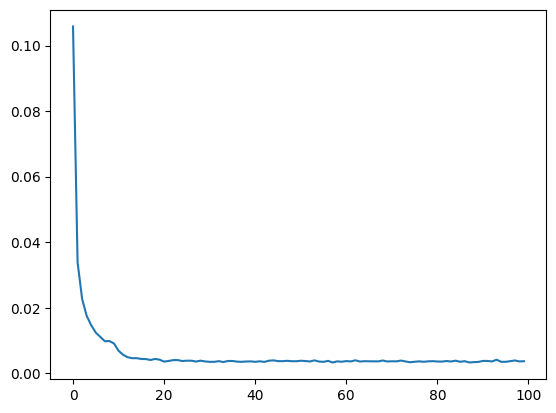
During the training, each epochs would take some time to get trained on and you can track the loss. Setting the Google Colab to the T4 GPU Configuration would save a lot of time and the process of training each epoch reduces dramatically.
# The losses are accessed from the training_result dictionary with 'losses'
plt.plot(training_result["losses"])
plt.show()
This plot() showcases successful model training, showing rapid initial improvement followed by gradual refinement. The model appears to be learning effectively, with no obvious signs of overfitting or instability in the training process.

outputs = []
labels = []
net.eval()
# loop over train dataset and get embedding for each image
with torch.no_grad():
    for first, second, dis, label in tqdm(trainLoader):
        # Appends the embeddings and labels to their respective lists
        outputs.append(net(first.to(device)).cpu().detach().numpy())
        labels.append(label.numpy())

# Converting the list into the numpy array
outputs = np.concatenate(outputs)
labels = np.concatenate(labels)
To Generate the 64 Dimension of the MNIST Training Set
encoded_data = []
labels = []

with torch.no_grad():
    for anchor, _, _, label in tqdm(trainLoader):
        output = model(anchor.to(device))
        encoded_data.extend(output.cpu().numpy())
        labels.extend(label.cpu().numpy())

# Both outputs and labels are converted to numpy arrays.
encoded_data = np.array(encoded_data)
labels = np.array(labels)
torch.no_grad() context to disable gradient computation, which is appropriate for inference. It iterates through the trainLoader, but only uses the anchor images and labels.
For each batch -
Passes the anchor images through the model to get embeddings.
Extends the
encoded_datalist with the model outputs (embeddings).Extends the labels list with the corresponding labels.
Seaborn Plot for Embedding
The utility function plot_umap uses UMAP to reduce the dimensionality of the encoded data to 2D, using cosine distance as the metric. The resulting 2D embeddings are combined with labels into a pandas DataFrame. It sets up a matplotlib figure and applies seaborn styling.
import seaborn as sns
import matplotlib.pyplot as plt
import pandas as pd

def plot_umap(encoded_data, labels, random_state=42):
    # Create UMAP embeddings
    mapper = umap.UMAP(random_state=random_state, metric='cosine')
    umap_embeddings = mapper.fit_transform(encoded_data)

    # Create a DataFrame for easy plotting
    df = pd.DataFrame({
        'UMAP1': umap_embeddings[:, 0],
        'UMAP2': umap_embeddings[:, 1],
        'Label': labels
    })

    # Set up plot style
    plt.figure(figsize=(12, 10))
    sns.set_style("whitegrid")
    sns.set_palette("deep")

    # Create scatter plot
    sns_plot = sns.scatterplot(
        data=df,
        x='UMAP1',
        y='UMAP2',
        hue='Label',
        palette='deep',
        legend='full',
        alpha=0.7
    )

    # Customize the plot
    plt.title('UMAP Projection of Encoded Data', fontsize=16)
    plt.xlabel('UMAP1', fontsize=12)
    plt.ylabel('UMAP2', fontsize=12)
    plt.legend(title='Labels', title_fontsize='13', fontsize='11', loc='center left', bbox_to_anchor=(1, 0.5))

    # Adjust layout
    plt.tight_layout()
    plt.show()

plot_umap(encoded_data, labels)

Here, You can easily distinguish between the digit with the various cluster. Each cluster here, represents one of the label from the MNIST Dataset.
You Can Refer to the Github Repository for the Data and the Code file - https://github.com/Hrishikesh332/Large-Multimodel-Guide/tree/main/M1%20Overview%20Multimodality%20MNIST
If you're looking for the Train and Test Dataset of the MNIST, you can refer to - https://www.kaggle.com/competitions/digit-recognizer
Research Paper:
A Simple Framework for Contrastive Learning of Visual Representations: https://arxiv.org/pdf/2002.05709v3
Multimodal Contrastive Training for Visual Representation Learning: https://openaccess.thecvf.com/content/CVPR2021/html/Yuan_Multimodal_Contrastive_Training_for_Visual_Representation_Learning_CVPR_2021_paper.html
Multimodal Contrastive Learning with LIMoE: the Language-Image Mixture of Experts: https://proceedings.neurips.cc/paper_files/paper/2022/hash/3e67e84abf900bb2c7cbd5759bfce62d-Abstract-Conference.html
Understanding Multimodal Contrastive Learning and Incorporating Unpaired Data: https://proceedings.mlr.press/v206/nakada23a.html
Identifiability Results for Multimodal Contrastive Learning: https://arxiv.org/abs/2303.09166
Mind the Gap: Understanding the Modality Gap in Multi-modal Contrastive Representation Learning: https://proceedings.neurips.cc/paper_files/paper/2022/hash/702f4db7543a7432431df588d57bc7c9-Abstract-Conference.html
Subscribe to my newsletter
Read articles from Hrishikesh Yadav directly inside your inbox. Subscribe to the newsletter, and don't miss out.
Written by

Hrishikesh Yadav
Hrishikesh Yadav
With extensive experience in backend and AI development, I have a keen passion for research, having worked on over 4+ Research work in the Applied Generative AI domain. I actively contribute to the community through GDSC talks, hackathon mentoring, and participating in competitions aimed at solving problems in the machine learning and AI space. What truly drives me is developing solutions for real-world challenges. I'm the member of the SuperTeam and working on the Retro Nexus (Crafting Stories with AI on Chain). The another major work focused on the technological advancement and solving problem is Crime Dekho, an advanced analytics and automation platform tailored for police departments. I find immense fulfillment in working on impactful projects that make a tangible difference. Constantly seeking opportunities to learn and grow, I thrive on exploring new domains, methodologies, and emerging technologies. My goal is to combine my technical expertise with a problem solving mindset to deliver innovative and effective solutions.