Hello fellow data engineers!

This week, we delve into intricacies of Apache Spark optimizations, exploring how transformations like groupBy(), join types, partitioning, and adaptive query execution (AQE) enhance the performance and efficiency of data processing. Let's get started right away!

How a groupBy() works?

Consider an orders.csv dataset of 1.1GB size.
We perform the following groupBy() transformation on order_status column, which has 9 unique values.

groupBy() triggers a wide transformation, so by default, 200 shuffle partitions get created.

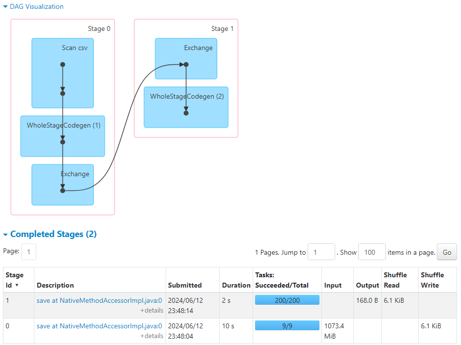
Since there are only 9 unique keys (in order_status), there would be only 9 partitions that have data, and the remaining 191 partitions remain empty.
The task scheduler gets overburdened to create tasks (~191) that would remain empty, without any data and don't perform any operations.

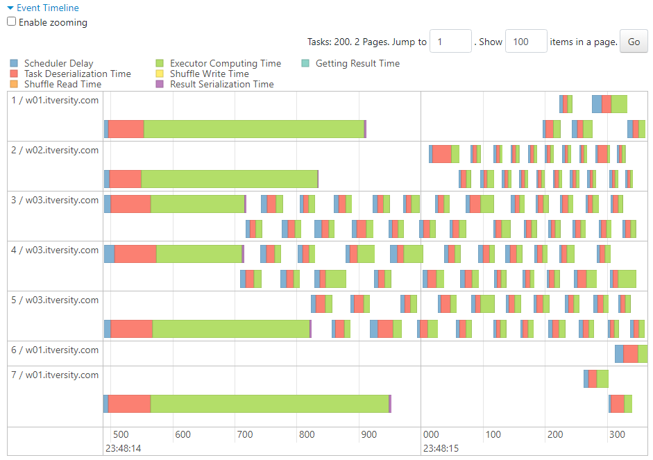
The data gets written into 9 files as follows.

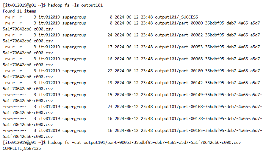
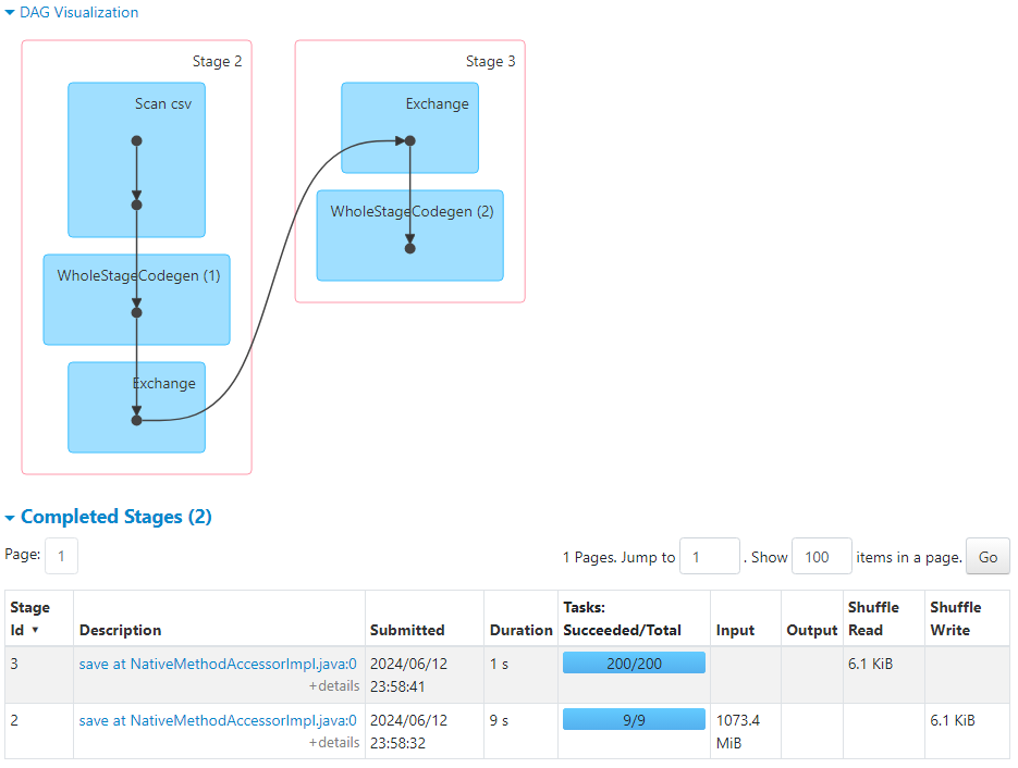
For testing purposes, we can use the following syntax since it does not write back to the disk.

This syntax also gives the same results.

Broadcast join & Normal shuffle-sort-merge join

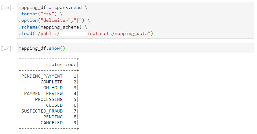
Consider the following two datasets: orders and customers.

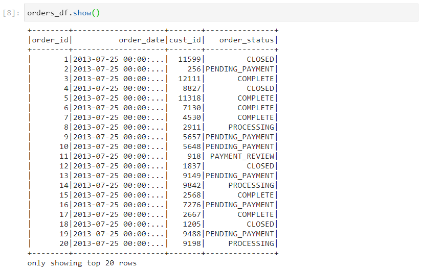
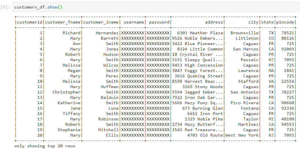
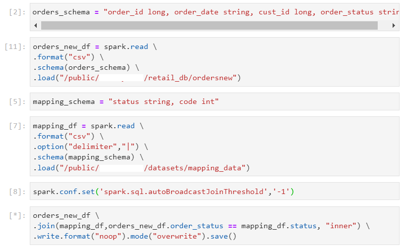
Firstly, let's set the threshold for broadcast join to a small value so that broadcast join does not happen for certain.

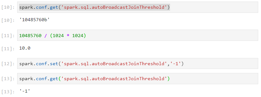
In the following example, customers dataframe is small and can be broadcasted across executors containing partitions of the large dataframe - orders.
For now, we have set the configurations in such a way that the smaller dataframe does not get broadcasted.

Following is the DAG visualization.

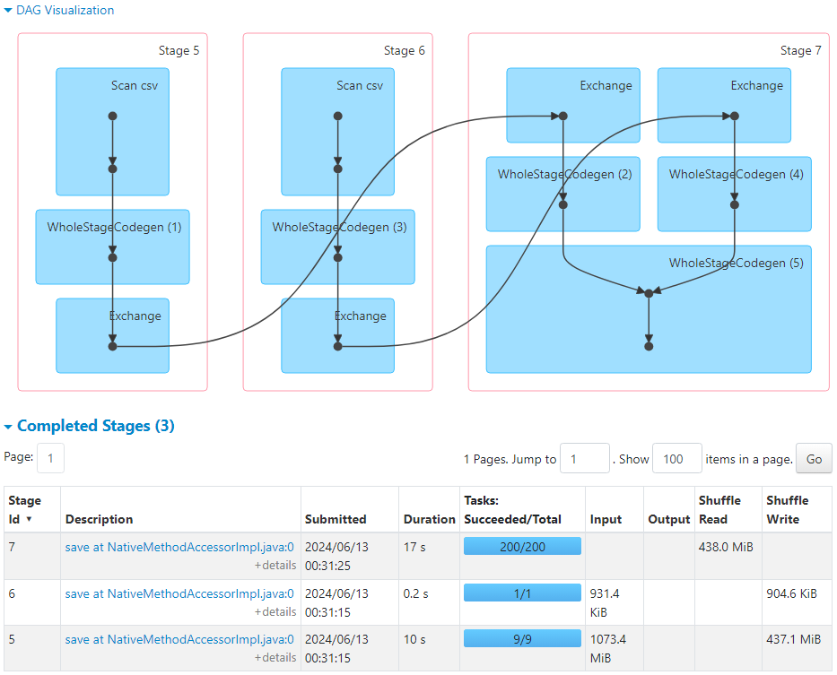
The following metrics indicate the average time taken by the tasks.

So, normal sort merge join takes place.

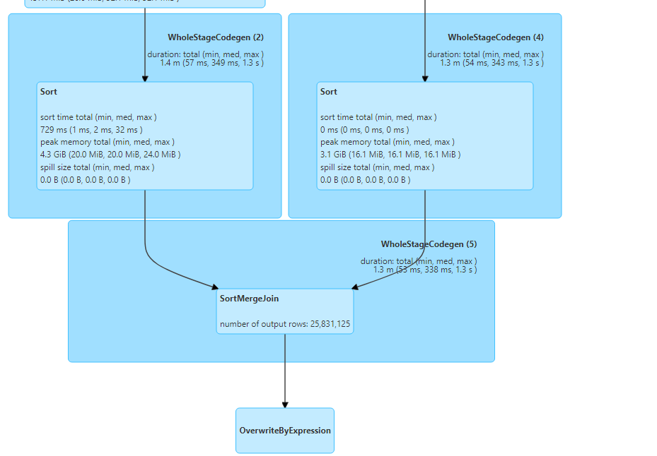
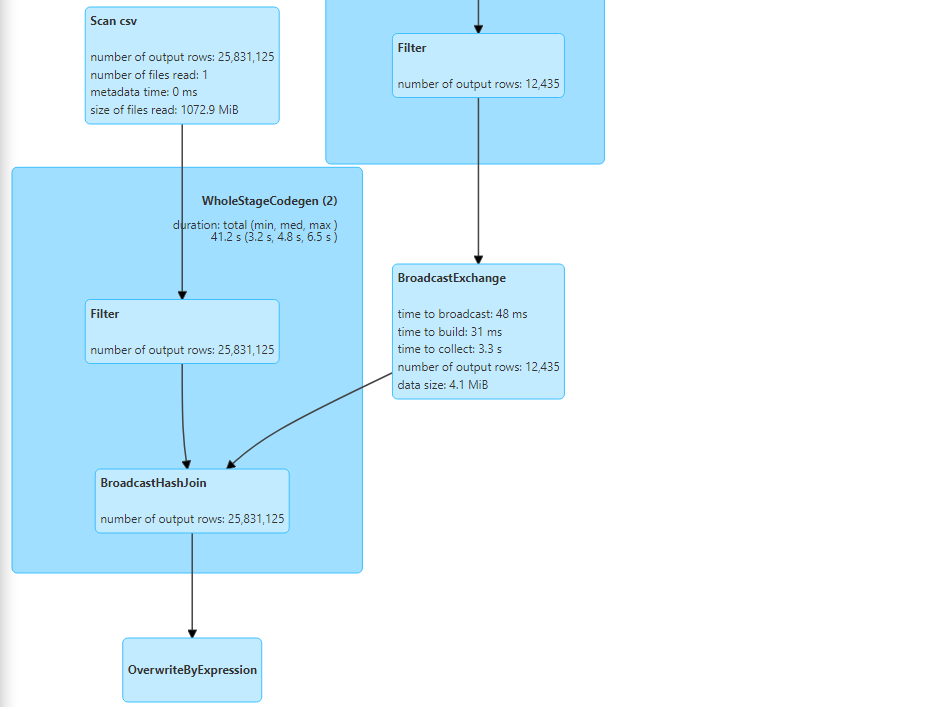
For broadcast join, let's set the threshold for broadcast join to a normal size.

If we perform the same query now,

Following are the DAG visualization and the number of tasks created.

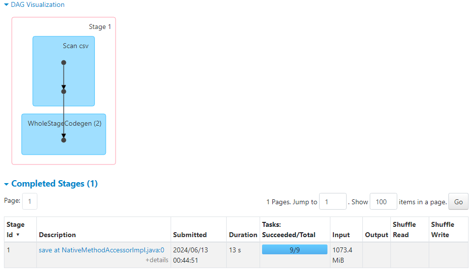
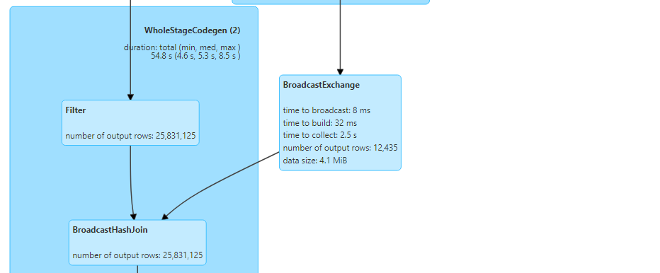
Hence, the customers dataset gets broadcasted and broadcast hash join takes place.

Join types

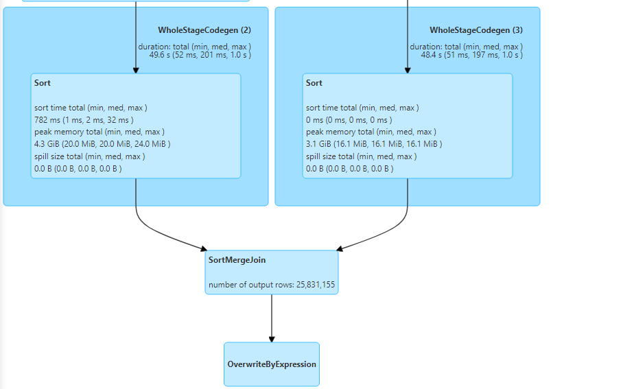
Right outer join: It gives all the matching records and the non-matching records from the right table.

Right outer join uses normal sort merge join in this case.

Left outer join: It gives all the matching records and the non-matching records from the left table.

Left outer join also uses normal sort merge join in this case.

Inner join: It gives matching records from both the tables.

Inner join uses broadcast hash join.

Partition skew

Partition skew occurs when one of the partitions holds relatively more data as compared to the rest of the partitions.
In the following example, COMPLETE has more data as compared to other order_status.

Consider the following dataset that needs to be joined with the orders dataset.

After ensuring that broadcast join does not happen, we perform the join operation.

Even though 200 partitions get created after shuffling in wide transformations, all the records with order_status 'COMPLETE' will still be moved to one single partition.
Due to this, one of the tasks takes significantly more time to complete and can also lead to out of memory error.

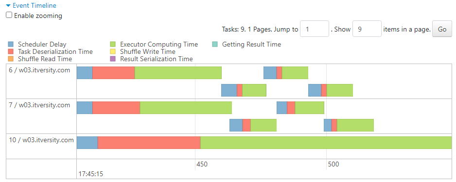
Partition skew leads to reduced parallelism. In our case, consider the executor with ID 10 with respect to others in the following image.

Adaptive query execution (AQE)

Earlier, Spark was not able to analyze the runtime statistics to improve the query performance by providing better optimization options.
In the following example, we try to join the orders data with distinct values of customers (less).

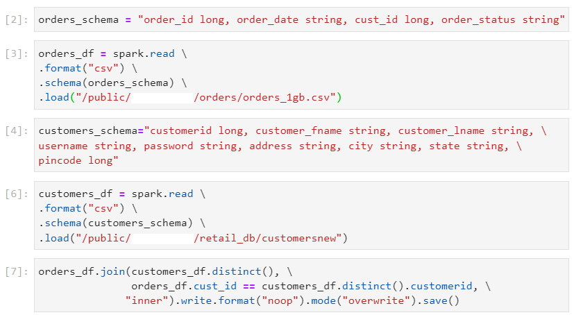
Despite the small number of unique customers, Spark would default to a time consuming shuffle-sort-merge join with 200 shuffle partitions.

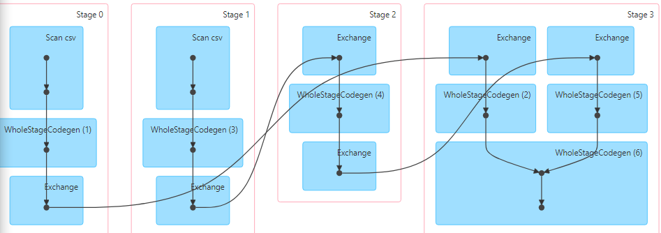
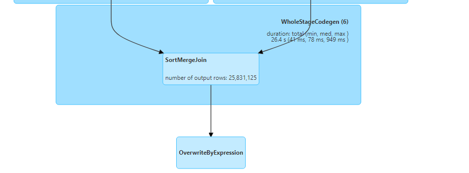
But now from Spark version 3, it can analyze runtime statistics and derive some insights like number of records, size of data, minimum and maximum of each column, number of occurrences of each key, etc.
The three major benefits resulting from AQE are as follows:

Dynamically coalescing the number of shuffle partitions

Firstly, we enable AQE as follows. Then, we perform the same groupBy() query as before.

Now, instead of 200, only 9 partitions get created.

The 9 tasks that get launched afterwards, get performed with optimal parallelism within executors.

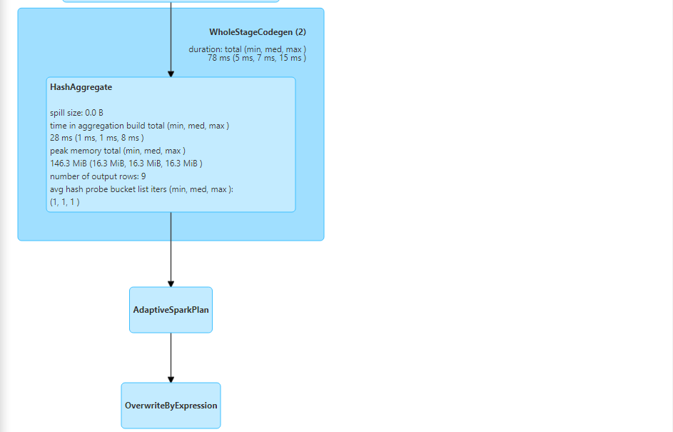
The enabling of adaptive query execution can also be determined by the query execution plan.

Dynamically handling partition skew

Consider the following scenario where AQE is not enabled.

Due to partition skew, one node gets overburdened.

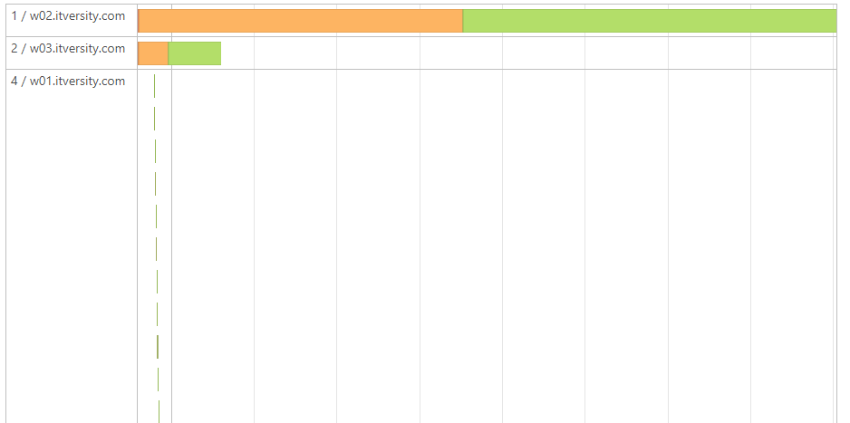
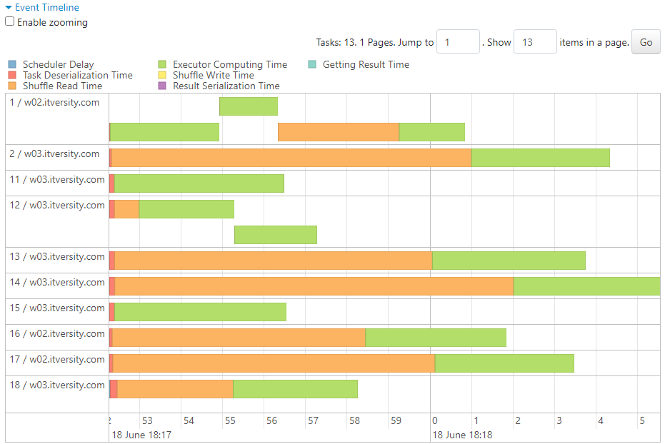
Now, we enable the AQE.

Upon performing the same query, optimal parallelism is achieved and partition skew is dealt with dynamically.

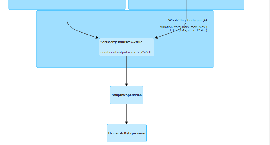
Adaptive Spark Plan indicates that AQE was indeed enabled.

Dynamically switching join strategies

Without enabling AQE, if we perform the join of customers dataset (small) with orders dataset (big), we get the following results.

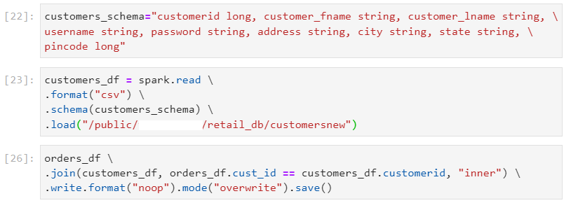
Normal sort merge join is performed, rather than the optimal broadcast join.

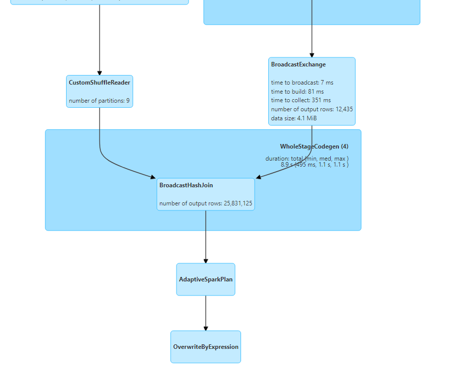
With AQE enabled, if we perform the same query on distinct customers, we observe as follows.

The join strategy gets switched dynamically and broadcast hash join is performed.

Join types

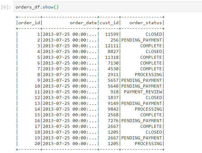
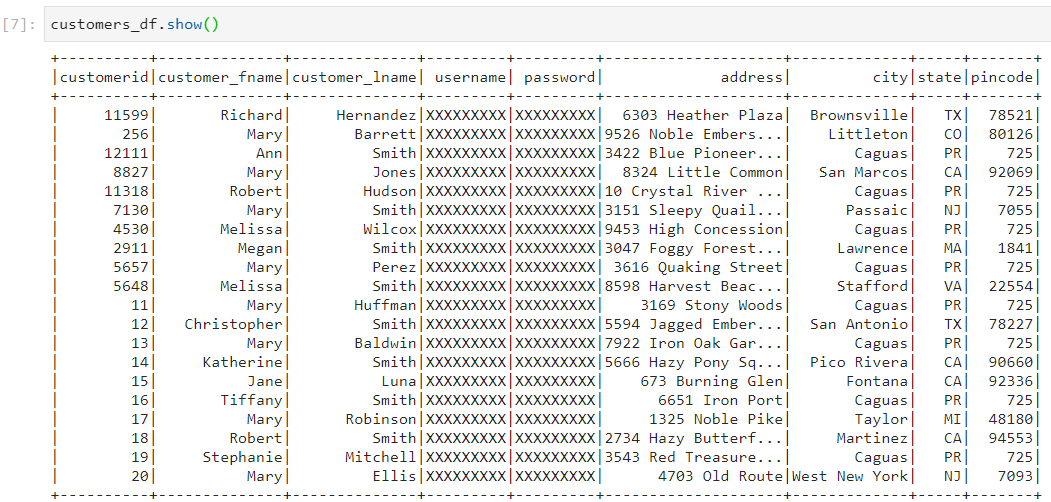
Consider the following orders and customers datasets.

Inner join: It gives matching records from both the tables, based upon the matching condition.

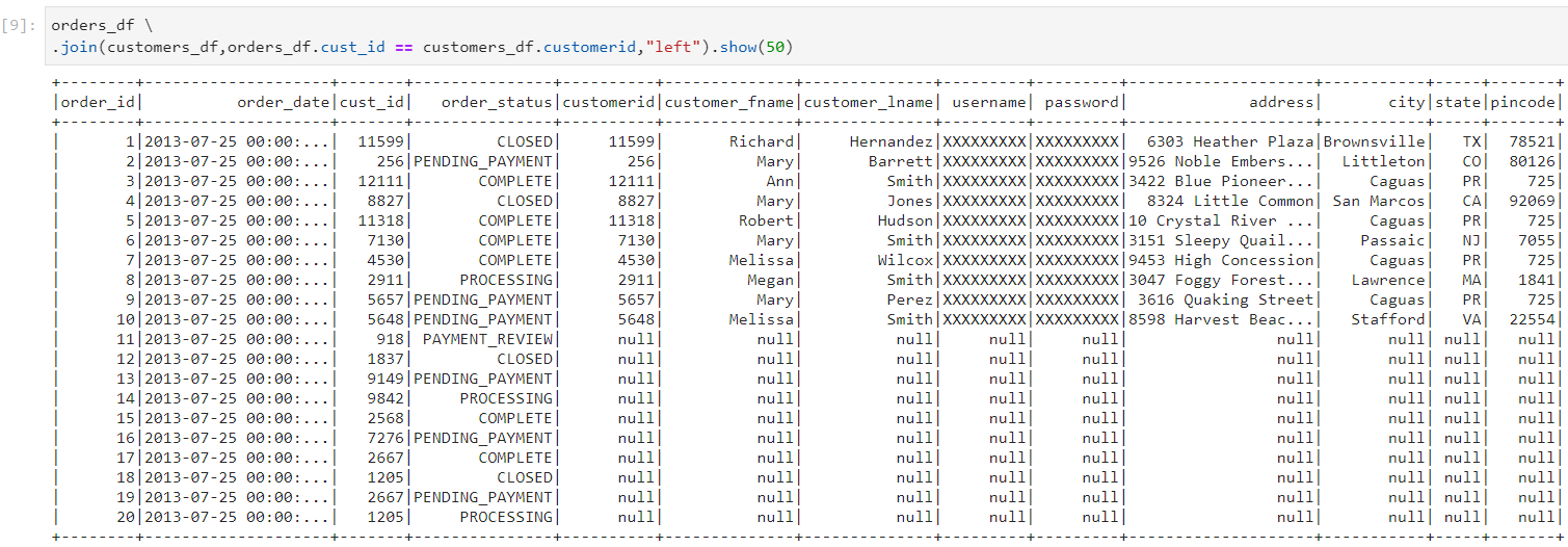
Left outer join: It gives matching records from both the tables, and also the non-matching records from the table on left side of the join. Corresponding values for the columns of the right table are filled with nulls.

Right outer join: It gives matching records from both the tables, and also the non-matching records from the table on right side of the join. Corresponding values for the columns of the left table are filled with nulls.

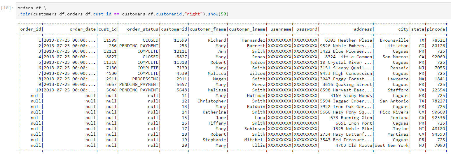
Full outer join: It is a combination of left outer join and right outer join. Along with matching records, it gives non-matching records from both the left and right tables.

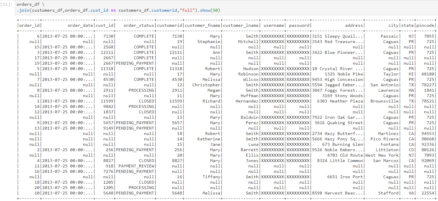
Left semi join: It only returns columns from the left-hand table, and yields one of each record from the left table where there is one or more matches in the right-hand table.
In the following example, we get the customers who have placed at least one order.

Left anti join: It returns all records from the left side that don't match any record from the right side.
In the following example, we get all the customers who have never placed any order.

Join strategies

Broadcast hash join

Since customers dataframe is small, Spark creates a hash table for it. The entire hash table is then broadcasted to all the executors consisting of partitions of the large orders dataframe.

The query execution plan indicates that broadcast hash join was performed, indeed.

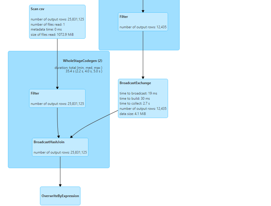
Moreover, broadcast hash join also gets specified in the physical plan of the query as follows.

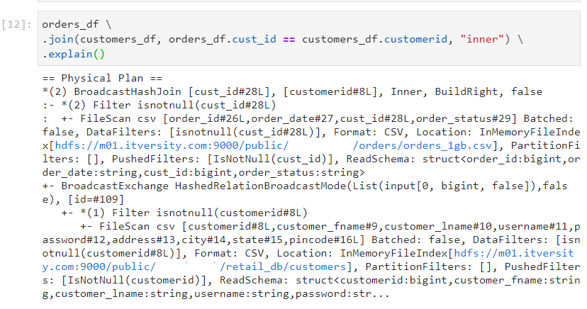
Shuffle sort merge join

It is the normal join and the physical plan for its query execution looks as follows.

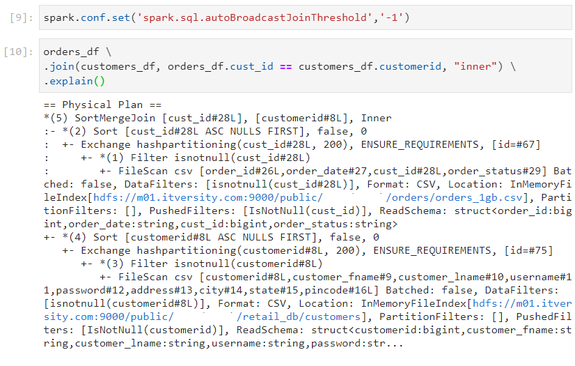
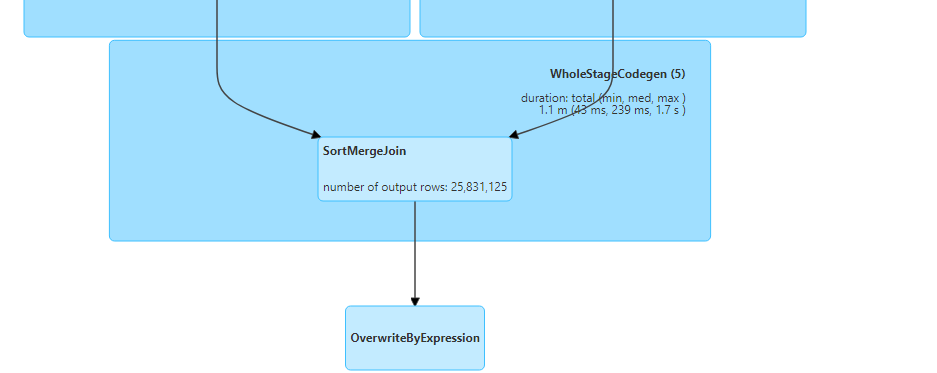
Visual representation for shuffle sort merge join.

Shuffle hash join

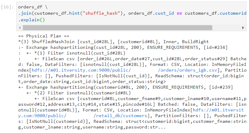
We need to explicitly provide the hint for shuffle hash join as follows.

The query execution looks as follows.

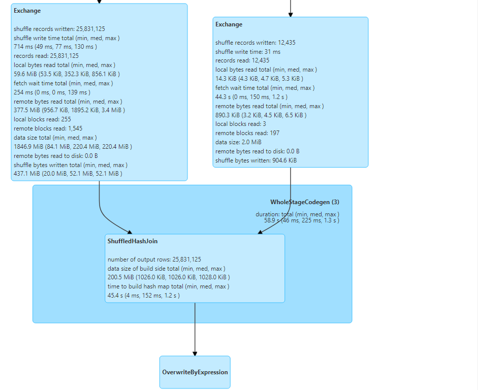
The physical plan further ascertains that shuffle hash join was performed.

Conclusion

Understanding the internal workings of Spark is crucial for optimizing data processing tasks. By leveraging techniques such as broadcast joins, partitioning, and adaptive query execution, you can significantly improve query performance and resource utilization. This knowledge not only boosts your data engineering skills but also ensures that your Spark applications run efficiently and effectively.

Stay tuned for more such blogs!

Week 7: Spark Optimization Unlocked 🔓