Introduction

Welcome to the 5th blog post in our machine learning series! Today, we will explore Support Vector Machines (SVM), a powerful and versatile algorithm used for both classification and regression tasks. As usual, we will also implement this algorithm from scratch in Python. By the end of this blog, you will have a solid understanding of SVM, its mathematical intuition, and when to use it.

Prerequisites

Hinge Loss: Penalizes predictions from the machine learning model that are wrongly classified. Think of it as a way to push the model to correct its mistakes.
Regularization: Helps to counter overfitting by penalizing larger weights. It keeps the model from becoming too complex and tailored to the training data.

What is SVM?

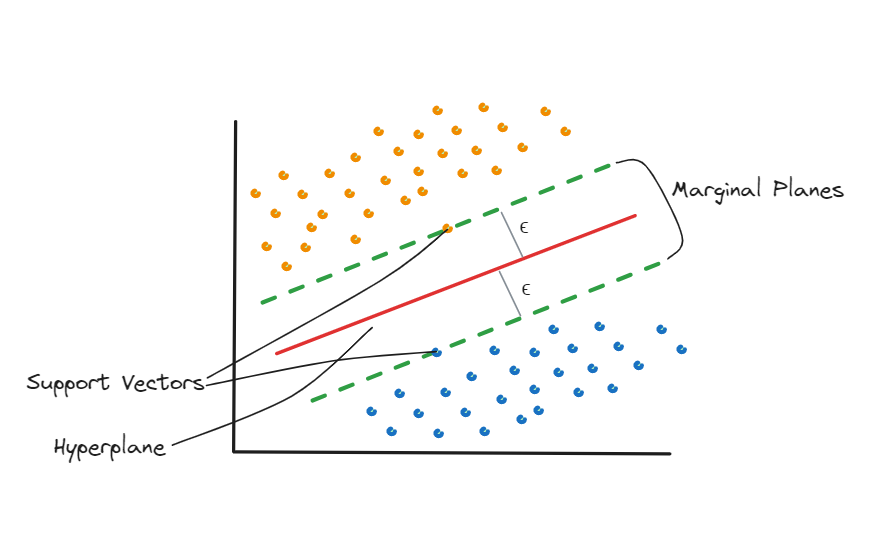
Support Vector Machine (SVM) is a supervised learning algorithm that can be used for both classification and regression tasks. It works by finding the best boundary (or hyperplane) that separates different classes of data points.

SVM for Regression and Classification

Classification

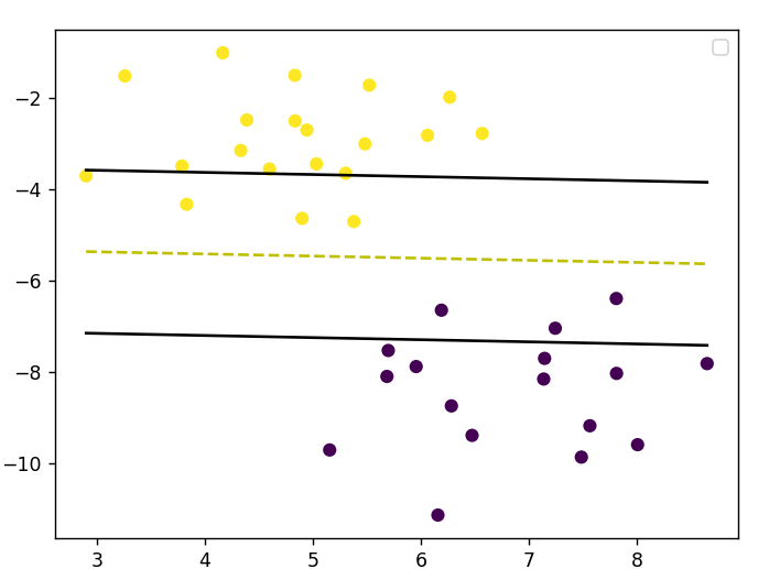
In classification, SVM finds the best fit hyperplane that separates the data into different classes. The best hyperplane is the one that maximizes the margin between the two classes. Think of the margin as a safe zone where no data points lie.

Regression

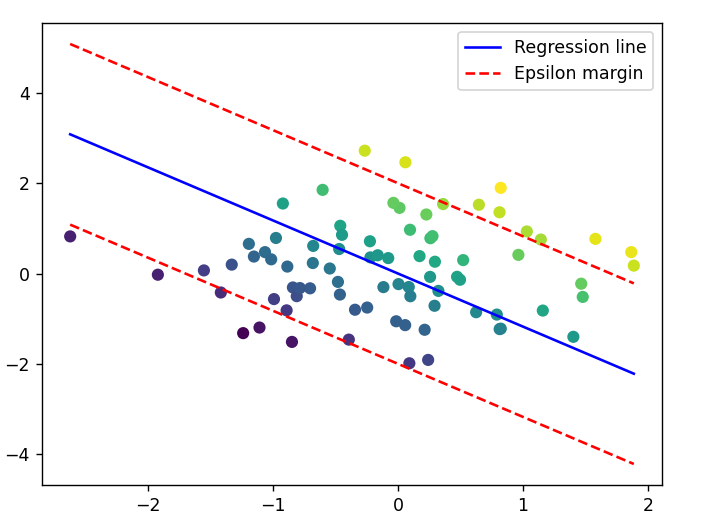
In regression, SVM tries to find a line that best fits the data points. Instead of maximizing the margin, SVM for regression uses a margin of tolerance (epsilon) within which it fits the line. The goal is to have as many points as possible under this margin.

Mathematical Intuition

For Classification

Objective:

SVM seeks a hyperplane that maximizes the margin between classes while minimizing classification errors.

Hyperplane Equation:

For linearly separable data, the hyperplane equation is:

$$w⋅x+b=0$$

Here,

w is the weight vector perpendicular to the hyperplane.
x represents the input vector.
b is the bias term.

The decision rule for classification is:

$$\begin{cases} 1 & \text{if } w \cdot x + b \geq 0 \\ -1 & \text{if } w \cdot x + b < 0 \end{cases}$$

Margin and Support Vectors

The margin is the distance between the hyperplane and the closest data points (support vectors) from each class. The goal of SVM is to maximize this margin.

For any point xi with label yi ∈ { −1, 1 }:

$$y_i (w⋅x_i + b)≥1$$

This ensures that the points are correctly classified and are at least a margin distance away from the hyperplane.

Maximizing the Margin

The margin is given by 2 / ||w||. We have to maximize the margin, or minimize ||w|| / 2.

Hinge Loss Function

SVM uses a hinge loss function to define the margin:

$$max(0,1−y_i (w⋅x_i +b))$$

Hinge loss is used in SVM because it effectively maximizes the margin between classes by penalizing misclassifications linearly based on their distance from the decision boundary.

This function penalizes misclassifications and encourages a wider margin between classes. It ensures that data points are correctly classified.

Example:

If a data point is correctly classified and far from the decision boundary, hinge loss is zero.
If a data point is on the wrong side of the boundary, hinge loss increases linearly with its distance from the boundary.

Regularization:

To prevent overfitting, SVM introduces a regularization parameter C. The objective function combines margin maximization and regularization:

$$min_{w,b} \frac{1}{2} ∣∣w∣∣^2+ \ \ C∑_{i=1}^n max(0,1−y_i (w⋅x_i +b))$$

Regularization helps ensure that the model generalizes well to new data.

Optimization:

Gradient descent iteratively adjusts w and b in the direction that minimizes the objective function. By computing gradients of the objective function with respect to w and b.

For Regression

Objective:

SVR aims to predict continuous values by fitting a hyperplane within a margin of tolerance (epsilon) around the true values.

Hyperplane Equation:

SVR predicts values using a hyperplane equation similar to classification:

$$w⋅x+b$$

Here, w and b are adjusted to minimize errors within the tolerance margin ϵ.

Margin Definition:

SVR uses an epsilon-insensitive loss function to define the margin:

$$max(0,∣y_i −(w⋅x_i +b)∣− \ \ ϵ)$$

This function allows errors within the margin ϵ to be ignored, focusing on errors outside the margin.

Regularization:

Similar to classification, SVR includes a regularization parameter C. The objective function balances margin maximization and regularization:

$$min_{w,b} \frac{1}2 ∣∣w∣∣^2 + \ \ C∑_{i=1}^n max(0,∣y_i −(w⋅x_i +b)∣− \ \ ϵ)$$

Regularization helps control the trade-off between fitting the data well and keeping the model simple.

Optimization:

Here we adjust w and b to minimize the epsilon-insensitive loss function. This process ensures the hyperplane fits the data within the tolerance margin ϵ, balancing accuracy and generalization.

Implementation Steps

You can find this code on my GitHub.

Initialization

We start by initializing the SVM class with various parameters like learning rate, regularization parameter, number of iterations, mode (classification or regression), and epsilon (for regression).

class SVM:
    def __init__(self, learning_rate=0.001, lambda_param=0.01, n_iters=1000, mode='classification', epsilon=0.1):
        """
        Initialization of SVM model with hyperparameters.
        Parameters:
        learning_rate (float): The learning rate for gradient descent.
        lambda_param (float): The regularization parameter.
        n_iters (int): Number of iterations for training.
        mode (str): 'classification' or 'regression'.
        epsilon (float): Epsilon value for epsilon-SVM regression.
        """
        if mode not in ['classification', 'regression']:
            raise ValueError("Mode must be 'classification' or 'regression'")
        self.lr = learning_rate
        self.lambda_param = lambda_param
        self.n_iters = n_iters
        self.weights = None
        self.bias = None
        self.mode = mode
        self.epsilon = epsilon

Training the Model

The fit method trains the model. For classification, it adjusts the weights and bias to maximize the margin. For regression, it minimizes the distance from the margin of tolerance.

    def fit(self, X, y):
        """
        Fits the SVM model to the training data.

        Parameters:
        X (numpy.ndarray): Training feature data.
        y (numpy.ndarray): Training labels.
        """
        n_samples, n_features = X.shape
        self.weights = np.zeros(n_features)
        self.bias = 0

        if self.mode == 'classification':
            y_ = np.where(y <= 0, -1, 1)
        else:
            y_ = y.copy()

        for _ in range(self.n_iters):
            for idx, x in enumerate(X):
                if self.mode == 'classification':

                    #* Cost Function: Regularized hinge loss function
                    #*                        n 
                    #* J = λ * ||w||^2 + 1/n (Σ max(0, 1 - Y(wx - b)))
                    #*                       i=1 

                    condition = y_[idx] * (np.dot(x, self.weights) - self.bias) >= 1
                    if condition:

                        #* J = λ * ||w||^2
                        #* ∇J = 2λw 
                        #* w = w - α(∇J)
                        #* b = b - α(0)

                        self.weights -= self.lr * (2 * self.lambda_param * self.weights)
                        self.bias = self.bias - self.lr * 0

                    else:
                        #* J = λ * ||w||^2 + 1 - Y(wx - b) 
                        #* ∇J = 2λw - yx
                        #* w = w - α(∇J) 
                        #* b = b - α(Y) 

                        self.weights -= self.lr * (2 * self.lambda_param * self.weights - np.dot(x, y_[idx]))
                        self.bias -= self.lr * y_[idx]
                else:
                    #* Cost Function: Regularized epsilon-insensitive loss function
                    #*                        n 
                    #* J = λ * ||w||^2 + 1/n (Σ max(0, |Y - (wx - b)| - ε))
                    #*                       i=1 

                    condition = np.abs(np.dot(x, self.weights) - self.bias - y_[idx]) <= self.epsilon
                    if condition:
                        #* J = λ * ||w||^2
                        #* ∇J = 2λw
                        #* w = w - α(∇J)
                        #* b = b - α(0)

                        self.weights -= self.lr * (2 * self.lambda_param * self.weights)
                    else:
                        #* J = λ * ||w||^2 + |y - (wx - b)| - ε
                        #* ∇J = 2λw - x * (Y - (w*x))
                        #* w = w - α(∇J)
                        #* b = b - α(Y - wx)

                        self.weights -= self.lr * (2 * self.lambda_param * self.weights - np.dot(x, y_[idx] - np.dot(x, self.weights)))
                        self.bias -= self.lr * (y_[idx] - np.dot(x, self.weights))

Making Predictions

The predict method is used to make predictions on new data.

    def predict(self, X):
        """
        Predicts using the trained SVM model.

        Parameters:
        X (numpy.ndarray): Test feature data.

        Returns:
        numpy.ndarray: Predicted labels or values.
        """
        approx = np.dot(X, self.weights) - self.bias
        if self.mode == 'classification':
            return np.sign(approx)
        else:
            return approx

Example: Classification

if __name__ == "__main__":
    #* Classification 
    X, y = datasets.make_blobs(n_samples = 50, n_features = 2, centers = 2, cluster_std=1.05, random_state=44)
    y = np.where(y==0,-1,1)
    X_train, X_test, y_train, y_test = train_test_split(X,y,random_state=44)
    classifier = SVM()
    classifier.fit(X_train, y_train)
    predictions = classifier.predict(X_test)
    print('Accuracy: ', accuracy(y_test,predictions))
    visualize_svm(X_train, y_train, classifier, 'classification')

Example: Regression

    #* Regression
    X, y = datasets.make_regression(n_samples=100, n_features=2, random_state=42)
    # Split the dataset into training and testing sets
    X_train, X_test, y_train, y_test = train_test_split(X, y, test_size=0.2, random_state=42)
    # Initialize the SVM regressor
    regressor = SVM(mode='regression', epsilon=2)
    # Fit the regressor to the training data
    regressor.fit(X_train, y_train)
    # Make predictions on the testing set
    predictions = regressor.predict(X_test)
    # Calculate and print the Mean Squared Error
    mse = mean_squared_error(y_test, predictions)
    print('MSE:', mse)
    visualize_svm(X_train, y_train, regressor, 'regression')

Common Misconceptions about SVM

SVMs are only for binary classification: SVMs can be extended to multi-class classification problems using strategies like One-vs-One or One-vs-All.
SVMs always use a linear kernel: While linear kernels are common, SVMs can use various kernels like polynomial, radial basis function (RBF), and sigmoid to handle non-linear relationships.
SVMs are not scalable: While SVMs can be computationally intensive, especially with large datasets, techniques like the Sequential Minimal Optimization (SMO) algorithm and using kernel approximation can help scale SVMs effectively.

When to Apply SVM

Small to medium-sized datasets: SVM works well in case of limited number of samples.
High-dimensional spaces: Effective when there are large number of features.
Clear margin of separation: Best when there is a clear gap between classes.

Advantages of SVM

Effective in high-dimensional spaces.
Versatile with different kernel functions.
Robust to overfitting in high-dimensional space.

Disadvantages of SVM

Not suitable for large datasets due to high training time.
Does not perform well when classes overlap significantly.

Conclusion

I really hope this guide is useful to you; if so, please like and follow. You may also check out my other blogs, which I have been posting in a series on machine learning algorithms. I hope you enjoy them. Kindly provide a remark if you found any errors or have any recommendations.

A Step-by-Step Guide to SVM in Machine Learning

Table of contents