Hey data enthusiasts! 👋

In this week's blog, we delve into Spark Performance Tuning, focusing on optimizing aggregate operations and understanding the intricacies of Spark's logical and physical plans. We explore how sort and hash aggregations differ, the importance of file formats, and the Catalyst optimizer's role in enhancing query performance. Get ready to unlock advanced Spark techniques to boost your data processing efficiency!

Sort aggregate vs Hash aggregate

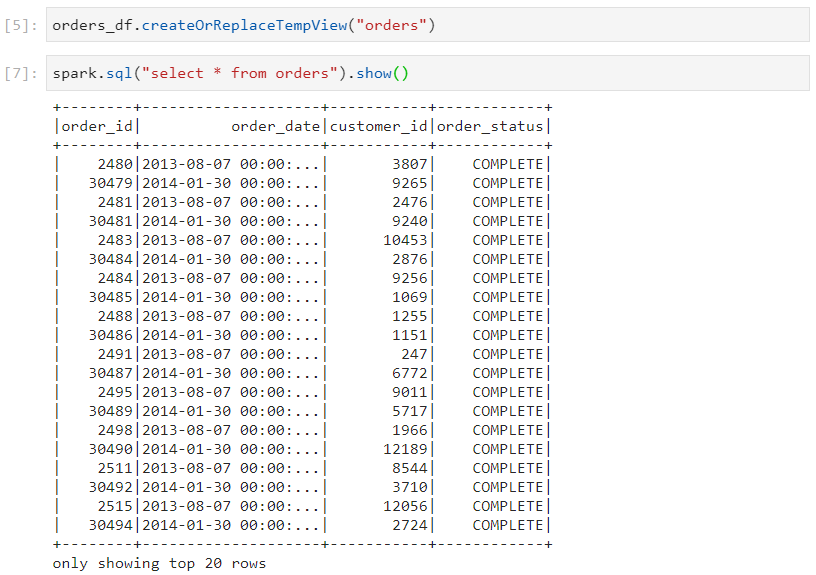
Consider the following orders dataset.

Scenario 1

We execute the following query:

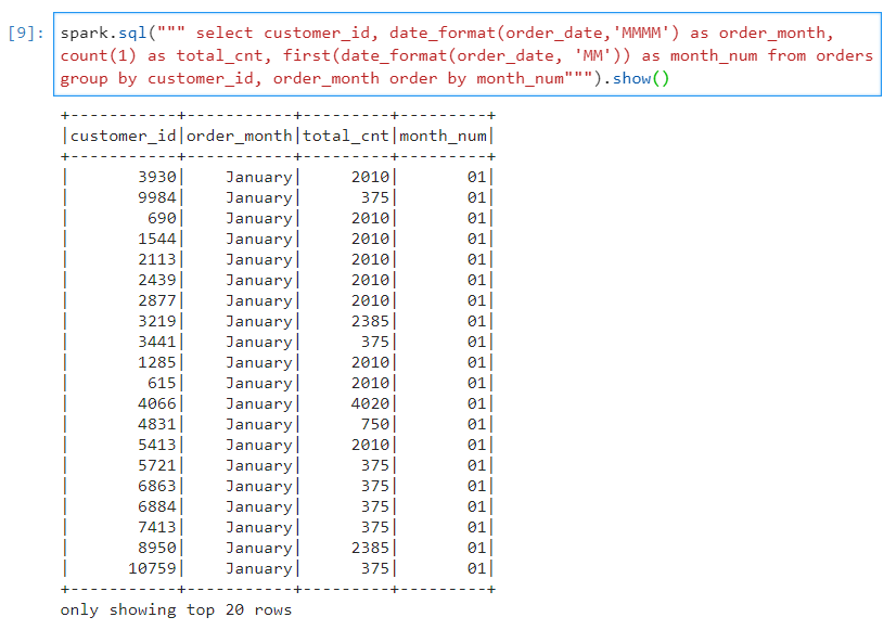
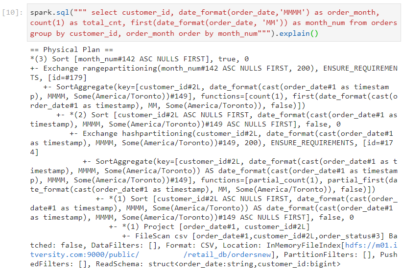
In order to get the execution plan without writing the results onto the disk, we use the following syntax for the same query.

This query took 1.1 minutes to complete.

As evident, sort aggregate takes place in this scenario.

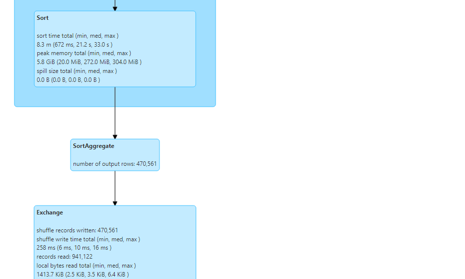
In sort aggregation, sorting of data happens before aggregation.
Sorting is quite a costly operation and takes a significant amount of execution time. Time complexity for sorting is O(nlogn).
The physical plan for the query confirms that sort aggregation took place, indeed.

Scenario 2

We execute the following query in which the only difference is that the month field has been changed into an integer.
Hash aggregate could not occur in scenario 1 because the datatype for month was string, and string is an immutable datatype.

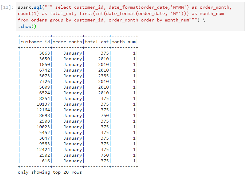
Syntax for observing the query execution plan without writing to the disk.

This query took only 25 seconds to complete.

As we can observe, hash aggregate takes place in this scenario.

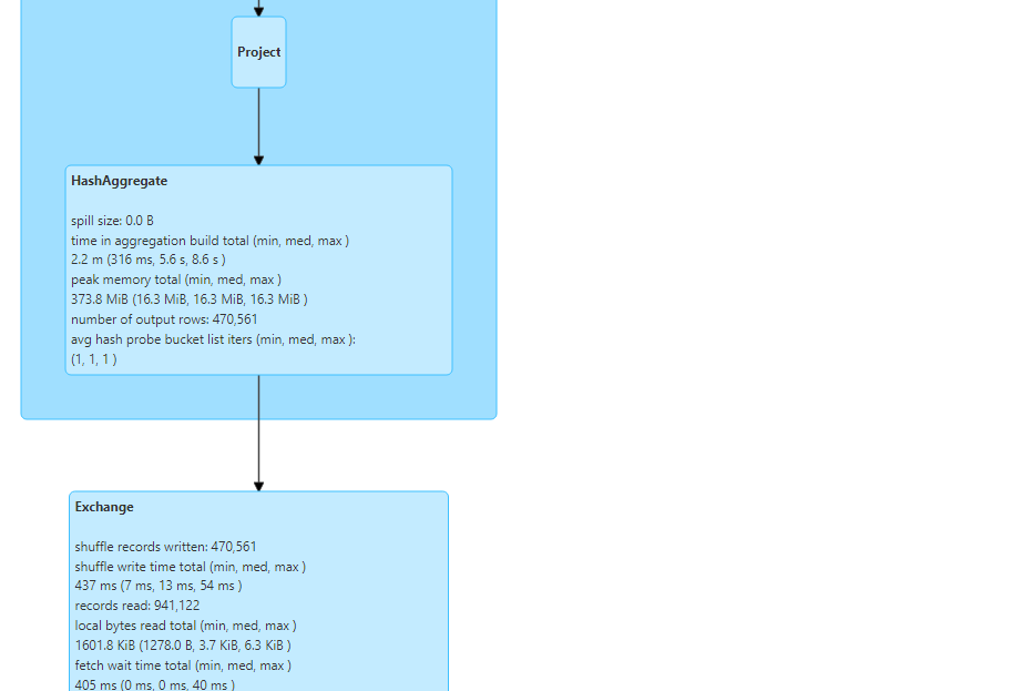
In hash aggregation, a hash table gets created which keeps getting updated based on the following two options:
1. If a new key is encountered , it gets added to the hash table.
2. If an existing key is encountered, it gets added to the value of the key in the hash table.
Time complexity of hash aggregate is O(n). But it requires additional memory for hash table creation.
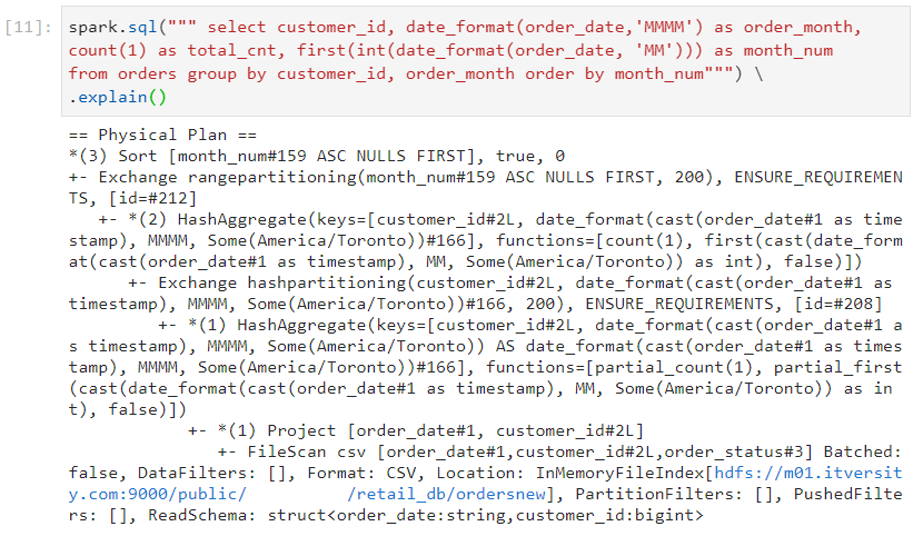
Hash aggregate can be seen in the physical plan as well.

Spark Logical and Physical plans

Parsed logical plan (Unresolved): Note that when we make a syntax error, parse exception takes place, indicating that syntax errors are handled by parsed logical plan.

Analyzed logical plan (Resolved): When we make a mistake in terms of the columns that need to be fetched, analysis exception takes place, indicating that such errors are handled by analyzed logical plan.

Consider that we have executed the following query.

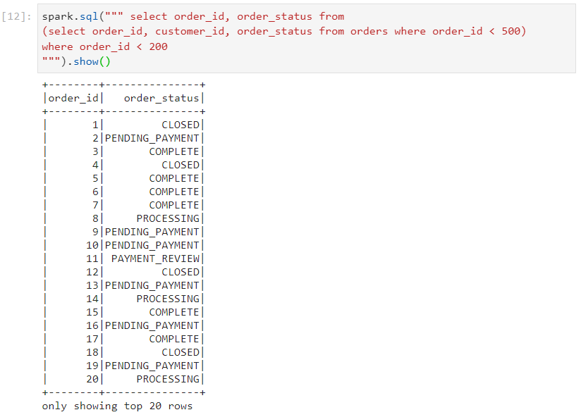
In order to fetch all of the plans, we execute the following query syntax.

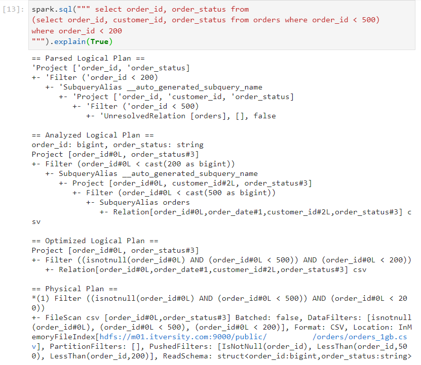
Optimized logical plan: Certain predefined rules are used to optimize the query execution plan at the early stages. Examples:
Consider the following query in which we join two datasets on the basis of a join condition.

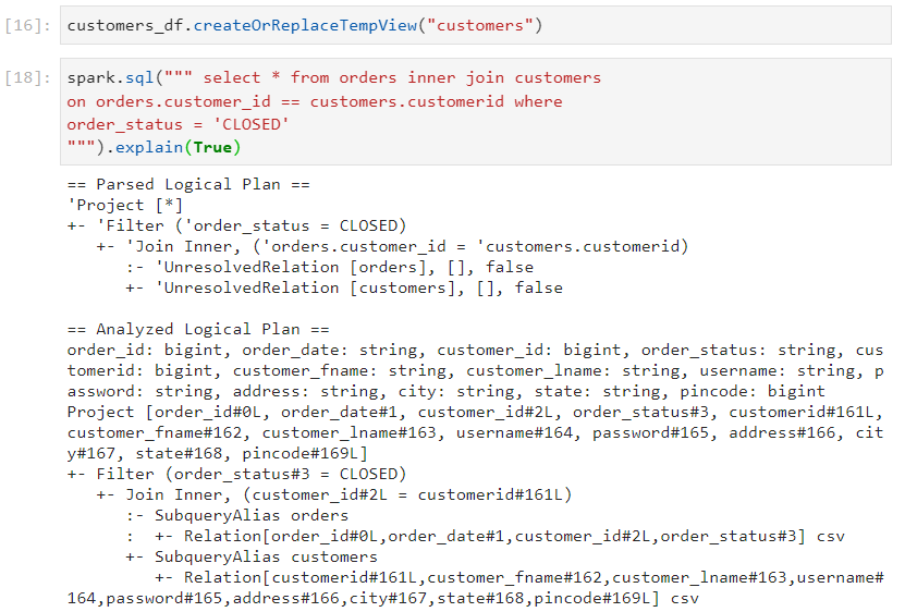
Optimized logical plan combines multiple filters into a single operation. This can be seen in the following image.

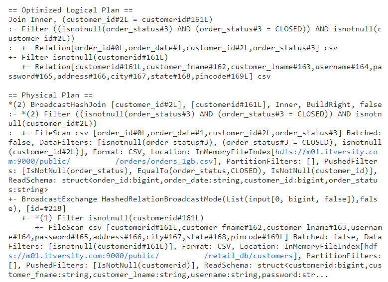
Physical plan: As we can observe in the above image, physical plan is used to decide join and aggregation strategies for optimal query performance.

Let's say we execute the following query.

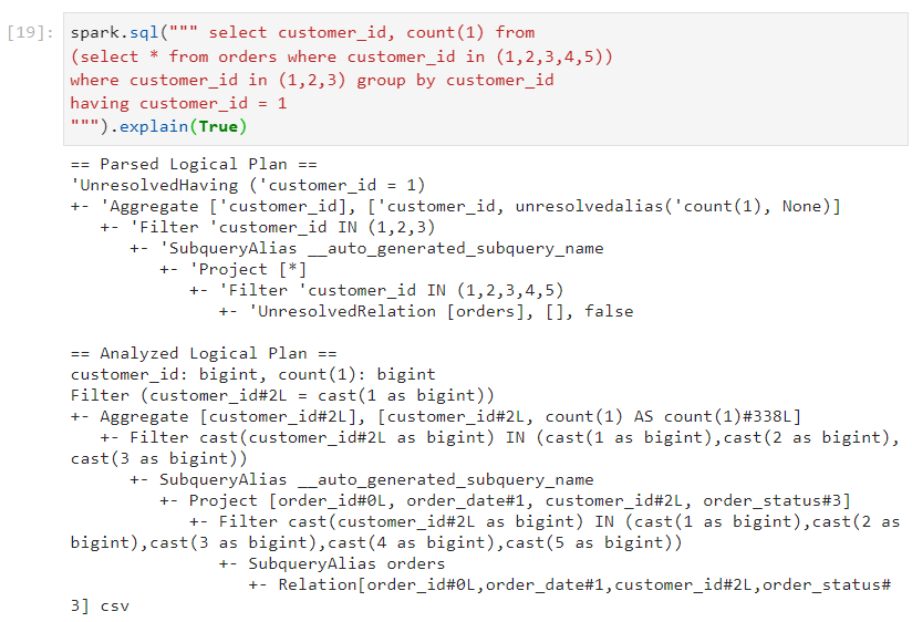
Predicate pushdown: In this case, the filters are pushed down so that they get applied at early stages, ensuring that operations are performed on the relevant data only.
Optimized logical plan also combines multiple projections into a single projection.

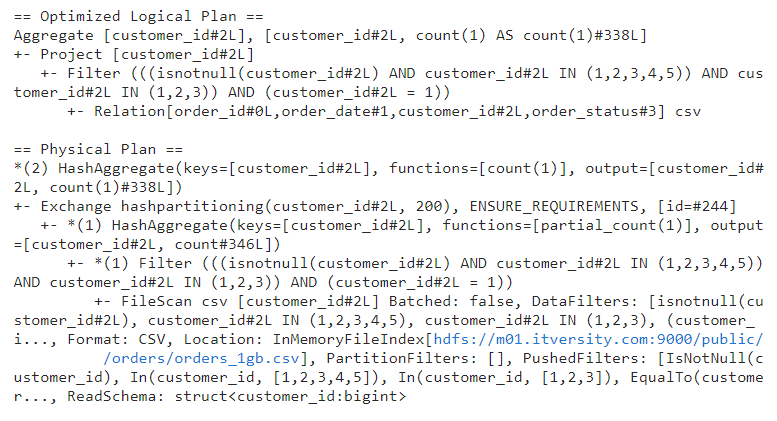
In the above image, physical plan determines whether to use hash aggregate or sort aggregate.

Catalyst optimizer

It refers to an optimization process where a particular query execution goes through a set of either pre-configured or custom-defined rules in the optimization layer to improve the query performance.
We use Scala syntax for the following example.

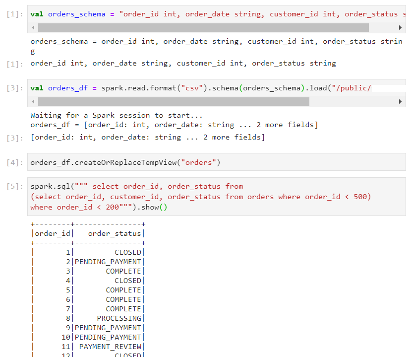
For the table orders, whether we write order_id or order_id*1, it does not make any difference in the result. But, this extra multiplication operation results into costly execution while projecting the result.

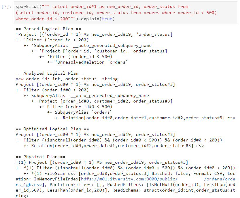
We need to define a custom rule by which if we have an operation: left * right and if the right side is 1, then we must ignore the multiplication.
We define the following custom rule using catalyst optimizer, in order to achieve the requirement.

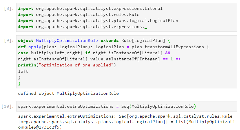
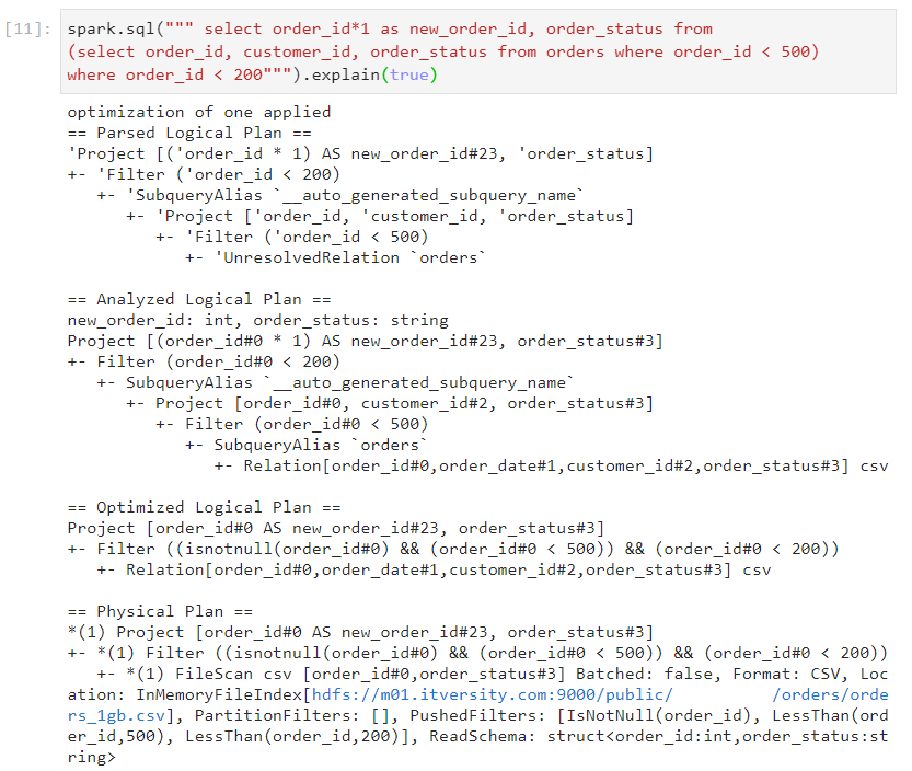
Now, if we perform the same query again, multiplication by 1 will be ignored in the optimized logical plan. We can observe it in the following image.

File formats

There are two broad categories of file formats:

Row based file format: The entire record i.e. all the column values of a row are stored together, followed by the values of the subsequent records.
- Used for faster writes as appending new rows is easy in this case.
- Provides slower reads as reading a subset of columns is not efficient.
- Provides less compression.
Column based file format: The values of a single column of all the records are stored together, followed by the column values of the next column.
- Used for efficient reading of a subset of columns as only the relevant data can be read without going through the entire dataset.
- Provides slower writes as data has to be updated at different places to write even a single new record.
- Provides good compression.

File formats not suitable for Big Data processing:

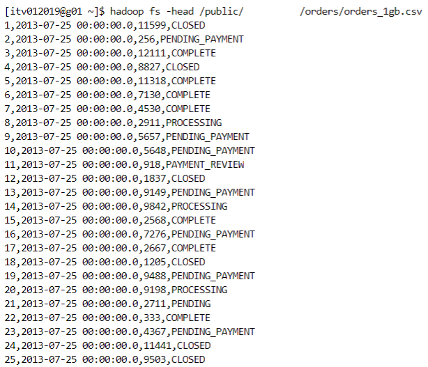
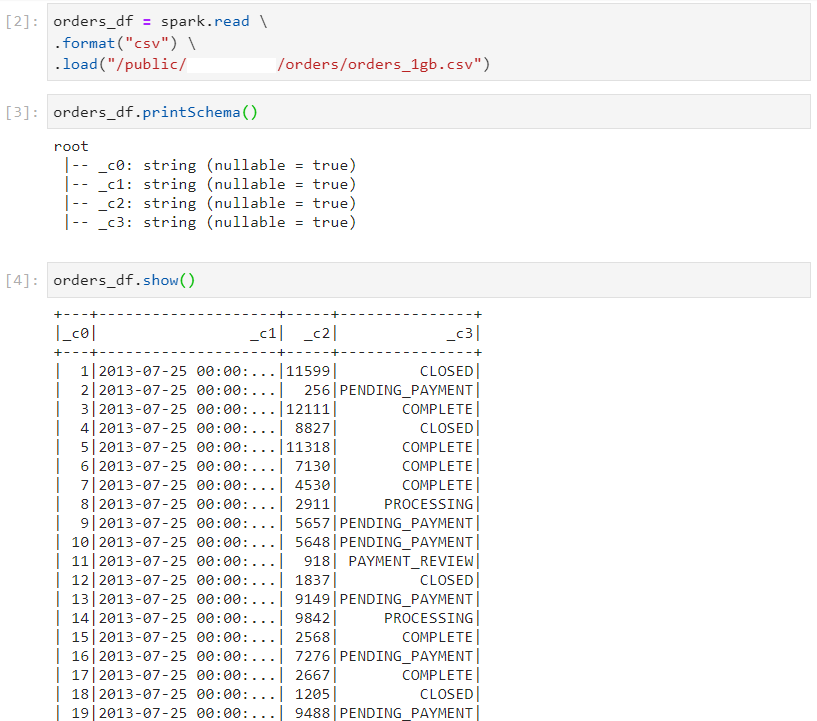
Text formats like CSV: Store the entire data as text, therefore consuming a lot of memory for storing and processing.

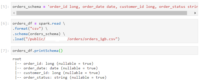
In order to perform different mathematical operations, strings need to be casted into required datatypes.

Casting / conversion is a costly and time consuming operation.

XML and JSON: These file formats contain partial schema.

All the disadvantages of text based file formats are applicable here as well.

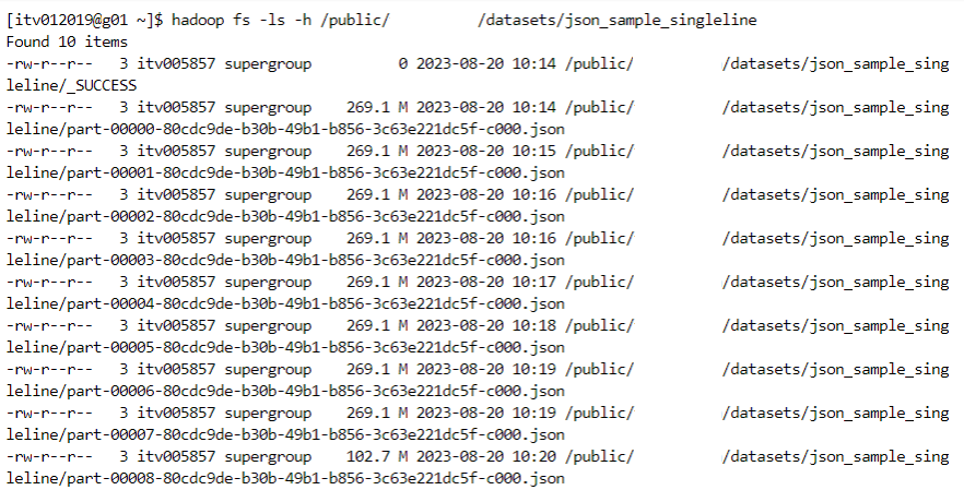
Since these have inbuilt schema associated with their data, these file formats are bulky.

A lot of input output operations to disks are involved in these file formats.

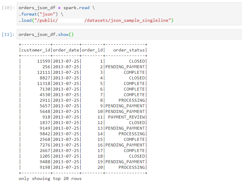
In the following JSON multiline example, we try to split the file.

We read the dataset as follows.

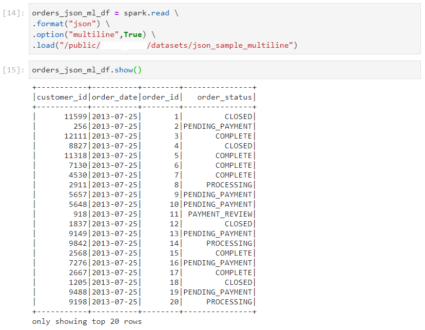
Even after reducing the maximum threshold for partition bytes, only 1 partition gets created, hence implying that JSON file format is not splittable. So, parallelism can not be achieved.

Specialized file formats for Big Data processing:

There are 3 main file formats well suited for Big Data problems:

AVRO:
- row based file format, splittable, supports schema evolution and supports all the compression techniques.
- best fit for storing data in the landing zone of Datalake.

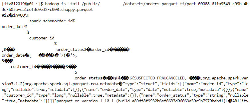
PARQUET:
- column based file format, supports schema evolution, splittable and supports all the compression techniques.
- most compatible with Spark.

ORC:
- column based file format, splittable, supports schema evolution and all the compression techniques.
- compatible with hive.

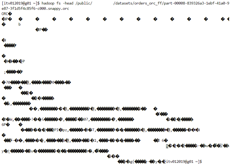
Schema evolution

Data evolves with the passage of time, requiring corresponding changes in the schema to be updated. Schema evolution allows for easy incorporation of the changes in the schema of this evolving data.
Some of the events that may cause the schema to change are: adding new columns, dropping existing fields, changing the datatypes, etc.
Consider the orders dataset with columns - order_id and order_date.

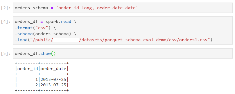
Consider other new orders dataset with columns order_id, order_date and customer_id, which is loaded into the dataframe and written in the parquet file format.
In order to enable the schema evolution feature, the property mergeSchema has to be enabled by using:
```
  option("mergeSchema",True)
```

Generalized Compression techniques

Snappy
- optimized for speed and gives moderate level of compression.
- default compression technique for PARQUET and ORC, splittable with these container based file formats.
- not splittable by default with CSV or text file formats.
LZO
- optimized for speed with moderate compression
- splittable by default
Gzip
- provides high compression ratio, therefore slow in processing
- splittable only when used with container based file formats
Bzip2
- most optimized for storage and provides best compression
- inherently splittable

Syntax for using the desired compression technique:

orders_df.coalesce(1).write.format("csv") \

.option("compression","snappy") \

.mode("overwrite").option("path","/public").save()

Conclusion

By mastering Spark's performance tuning techniques, you can significantly enhance the efficiency and speed of your data processing tasks. Understanding the difference between sort and hash aggregation, the impact of file formats, and leveraging the Catalyst optimizer are key steps in this journey. Implement these strategies to achieve optimal performance and make the most of your big data workflows.

Stay tuned!

Week 8: Spark Performance Tuning 🎶