Can we improve quantization by fine tuning?
 RJ Honicky
As a followup to my previous post Are All Large Language Models Really in 1.58 Bits?, I've been wondering if we could apply the same ideas to post-training quantization. The authors trained models from scratch in The Era of 1-bit LLMs: All Large Language Models are in 1.58 Bits and found that they were able to train models that perform at the same level of quality as full precision models using a few tricks, including ternary (-1,0,1) weights, weight-only quantization (e.g. don't quantize embeddings, activations, biases or other parameters), and "passthrough" weight updates (e.g. use full precision in the backward pass during training).
The passthrough weight update mean that the technique they describe in the paper has to be applied during training, so we can't apply the technique to existing models (e.g. Llama 3, Mixtral, Phi-3) that we know and love. On the other hand, if we continue training a model on data from the distribution of data in the original training, but with quantization during the forward pass, then perhaps we can reach a minimum with respect to the loss function that is close by the un-quantized minimum.
Post training quantization
Post training quantization does poorly at higher quantization levels. From BitNet: Scaling 1-bit Transformers for Large Language Models (by the same authors):
This table doesn't really reflect the state of the art, however. The current state of the art post-training quantization seems to be auto-round, which uses an optimizer to improve how to round during quantization.. It does well for 4-bit quantization on a low_bit_open_llm_leaderboard that the authors created, but performance falls off at higher quantizations.
This is encouraging: this suggests that there are local minima in quantized space that are nearby the unquantized minima. The authors of the paper about the algorithms used by auto-round, Optimize Weight Rounding via Signed Gradient Descent for the Quantization of LLMs, state that
...we still observed a noticeable gap in the accuracy performance of ultra-low bit quantization compared to the original model, such as 2-bit quantization. This challenge could potentially be addressed by exploring non-uniform quantization and mixed-precision quantization
It seems likely (to me) that if the techniques they mentioned might find a good minimum in quantized weight space, then perhaps "just" continued pre-training would using a quantized forward pass might work as well.
Passthrough gradient
Again, one of the important tricks the 1.58-bit authors play is to quantize during the forward pass but maintain full precision in the backward pass (e.g the so-called “passthrough gradient”), as mentioned above.
I’m very inexperienced, so before I jump in with both feet, I want to get familiar with the tools and ideas using a toy model that is easy to visualize. Instead of using a language model, lets try quantizing using the same technique, but with simple model that finds a polynomial fit to a set of random points. Here is a notebook that I used to do some quick experiments: bitnet_1_58b_experiments.ipynb.
Toy problem: polynomial fit
Here an example polynomial fit which I've normalized to be in both the domain and range [0,1]:
It takes about 6 minutes to generate a 2 million of these with which to train the network (using unoptimized python).
A simple network
I'm going to learn to map from 7 random points to 100 outputs representing the polynomial fit. I used GELU for stability during training, and three hidden layers, because ...it seems to work fine.
PolynomialFitNetwork(
  (linear_gelu_stack): Sequential(
    (0): Linear(in_features=14, out_features=512, bias=True)
    (1): GELU(approximate='none')
    (2): Linear(in_features=512, out_features=512, bias=True)
    (3): GELU(approximate='none')
    (4): Linear(in_features=512, out_features=512, bias=True)
    (5): GELU(approximate='none')
    (6): Linear(in_features=512, out_features=512, bias=True)
    (7): GELU(approximate='none')
    (8): Linear(in_features=512, out_features=200, bias=True)
  )
)
Notice that that we have 200 output features. We will learn both the x and y output values, even though the x are just grid points, and easily learned. I decided to do this because I wanted some easy parameters to learn, so that there is some "sparsity" in the network, meaning that the network is compressible and therefore can lose precision in the weights and still work well. The point is
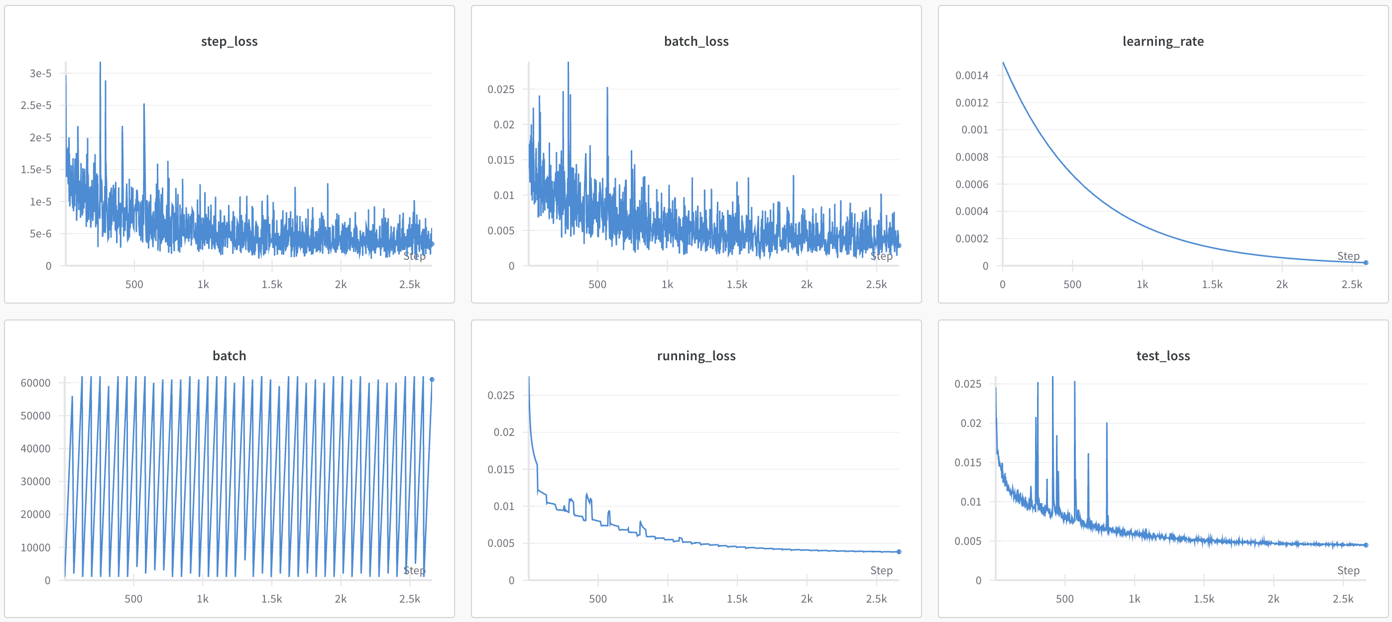
I trained for 41 epochs and got the test loss down to about 0.0045 (FWIW)

Lets take a look at some test examples
Some things I notice about these examples:
The blue line (the output from our model) doesn't necessarily pass through the points the function is fit to. This makes sense, since it is not a criterion in our loss function.
The model seems to struggle most when the variance of the input is high, and is good at predicting the values if the swing is very wide. Surprisingly, the model is good at predicting very wide swings precisely.
None of this is particularly important, except to illustrate that the problem is non-trivial for this neural network to solve.
Now quantize!
So now, lets define a quantized model and load the weights and see how we do.
Here's the code I used for BitLinear , adapted from https://huggingface.co/1bitLLM/bitnet_b1_58-3B/blob/main/utils_quant.py:
def weight_quant_158b(weight, num_bits=1):
    dtype = weight.dtype
    weight = weight.float()
    s = 1 / weight.abs().mean().clamp(min=1e-5)
    result = (weight * s).round().clamp(-1, 1) / s
    return result.type(dtype)

def weight_quant(x, num_bits=8):
    dtype = x.dtype
    x = x.float()
    Qn = -2 ** (num_bits - 1)
    Qp = 2 ** (num_bits - 1) - 1
    s = Qp / x.abs().max(dim=-1, keepdim=True).values.clamp(min=1e-5)
    result = (x * s).round().clamp(Qn, Qp) / s
    return result.type(dtype)

def activation_quant(x, num_bits=8):
    dtype = x.dtype
    x = x.float()
    Qn = -2 ** (num_bits - 1)
    Qp = 2 ** (num_bits - 1) - 1
    s = Qp / x.abs().max(dim=-1, keepdim=True).values.clamp(min=1e-5)
    result = (x * s).round().clamp(Qn, Qp) / s
    return result.type(dtype)


class BitLinear(nn.Linear):

    def __init__(self,
            *kargs,
            weight_bits=1,
            input_bits=8,
            **kwargs
        ):
        super(BitLinear, self).__init__(*kargs, **kwargs)
        """
        RMSNorm is placed outside BitLinear
        """
        self.weight_bits = weight_bits
        self.input_bits = input_bits

    def forward(self, input):

        if self.weight_bits == 1.58:
          quant = weight_quant_158b
        else:
          quant = weight_quant

        # quant_input = input + (activation_quant(input, self.input_bits) - input).detach()
        quant_weight = self.weight + (quant(self.weight, self.weight_bits) - self.weight).detach()

        # out = nn.functional.linear(quant_input, quant_weight)
        out = nn.functional.linear(input, quant_weight)

        if not self.bias is None:
            out += self.bias.view(1, -1).expand_as(out)

        return out
I combined support for quantization by any natural number of bits and ternary (1.58 bits). I also disabled the activation (input) quantization, because I want to focus on the impact of weight quantization for this toy model and I think that the activation quantization was peripheral in the paper.
Lets see how well we do with a 1.58-bit quantization. First we load the weights into a quantized model:
bit_model = BitPolynomialFitNetwork(weight_bits=1.58).to(device)
bit_model.load_state_dict(model.state_dict())
Lets see what our polynomials look like before training:
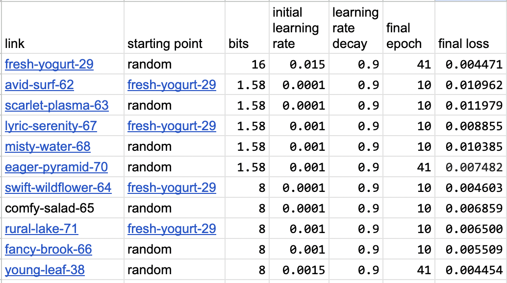
Oh man, that's pretty bad. Ok, lets try continued pre-training on the quantized model. We can try learning rates starting 1e-3 and 1e-4 with 1.58 bits and 8 bits for 10 epochs each to get a sense of how learning rate impacts the test loss. Here is a table:

I've added 41-epoch runs for 1.58 bits and 8 bits so that we can get a sense for the best we can expect to do at a give level of quantization. At 8-bits, we actually do slightly better than at 16 bits (probably not significant), but at 1.58 bits, we only get down to 0.007482, or about 67% greater loss. So maybe All Polynomial Fit Models Are Not In 1.58 Bits?
In any event, the 1.58b model that started at learning rate 1e-3 (lyric-serenity-67) seems to have reached a reasonably low loss of 0.008855 after 10 epochs; much better than the corresponding random run at 0.010385. The effect is even more pronouced at 8 bit, with the continued pre-training model starting at learning rate 1e-4 (swift-wildflower-64) reach a loss of 0.004603, and basically reaching the lower limit we estimated, whereas the corresponding random-init model only reaches 0.006500.
Learning rate and convergence
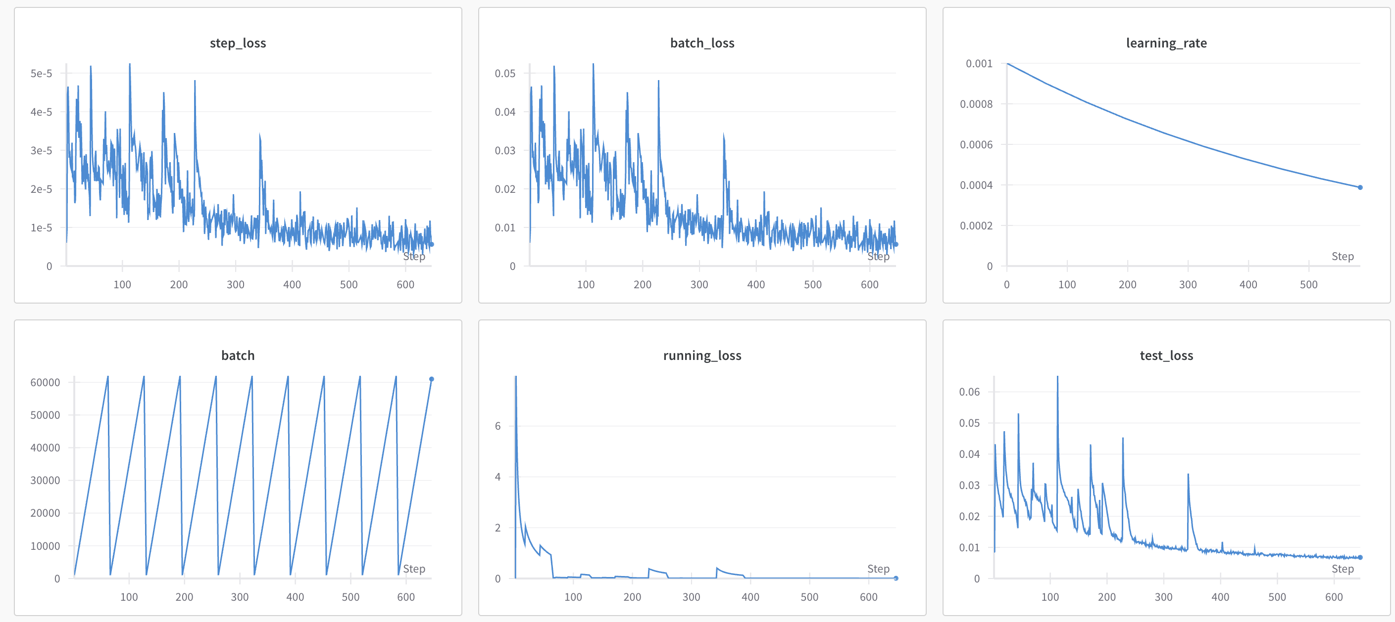
In many cases, I observed that higher learning rates caused instability (as is often the case). For example, from rural-lake-71, it looks like the instability is impacting the time to convergence.

Presumably we would continue to improve if we continued training, but the point here is to converge quickly.
Takeaways
Here are some things I learned from this experiment
At least for this toy model, fine-tuning (continued pre-training) a quantized model seems to be faster than starting from scratching
The training process seems to have different sensitivity to learning rate depending on the level of quantization. This is also consistent with the paper, in which they mentioned that more aggressive quantization needed higher learning rates in the beginning of the training process.
This is quite encouraging!
But wait... QALoRA?
Oh man! Here is an exciting paper: EfficientDM: Efficient Quantization-Aware Fine-Tuning of Low-Bit Diffusion Models. The authors have done something similar to my proposal, only
they fine-tuned a quantized diffusion model instead of an LLM. Some of the techniques they use may not be relevant, but
they used a quantized LoRA during fine tuning instead of fine tuning the whole model... brilliant! The LoRA can find the local minimum, and also
they use the un-quantized model to generate in-distribution data for training - another idea I had planned to use!
Awesome! They've paved the way! They call their technique Quantization Aware LoRA, or QALoRA.
I'm excited to try this idea on my toy model to see how much performance increase we get, and then implement it on a small language model.
The pythia family of models have Huggingface transformers versions that we can test these ideas on by making some minor changes to the GPTNeoXPreTrainedModel implementation to use our BitLinear implementation (with RMSNorm too, as in the paper).
I'll get working on it and write it up ASAP!
Subscribe to my newsletter
Read articles from RJ Honicky directly inside your inbox. Subscribe to the newsletter, and don't miss out.
Written by
