Guide to Principal Component Analysis in Data Science

1. Origin of PCA

2. Approach of PCA

3. How to do PCA

4. When is PCA used

5. What PCA is and is not

6. Advantages and Disadvantages of PCA

7. Metric of Evaluation

8. After PCA, what Next?

9. Case Study of the Cocktail recipe Dataset

---

Origin of PCA

PCA was first developed by Karl Pearson in 1901 and later developed by Hotelling in 1933.Pearson was a statistician and what he was working on when he developed PCA isn't entirely documented but we can suggest two things that could have prompted the development of the mathematical technique which are:

• Biometry(The application of Statistical methods to Biology)

• Factor Analysis

PCA applies an Orthogonal linear transformation to reframe the original correlated data in a new coordinate framework called Principal Components which are linearly uncorrelated. The largest variance(at least 80%) is usually explained in the First Component i.e. PC1 and the least component has the least Variance

Approach of PCA

There are two main approach of the PCA which are:

• Eigenvalue decomposition of the data covariance matrix

• Singular-Value Decomposition of the centered Data matrix

PCA is commonly used when many of the variables are highly correlated with each other and it's desirable to reduce their number to an independent set, the idea of PCA is to reduce the number of variables of a dataset while preserving as much information as possible

How to do PCA

This steps are done in the backend of the tool used to create the Principal Components

1. Standardize the range of continuous initial variables

2. Compute the covariance matrix to identify correlation

3. Compute the Eigenvalues and Eigenvectors of the covariance matrix to identify the Principal Components

4. Create a feature vector to decide which Principal Components to keep

5. Replot the data along the PC axes

When is PCA used?

PCA is used when we wish to reduce the dimensionality of a large dataset to a small and explains important information in the data

What PCA is and isn't

PCA is:

1. Is a Mathematical Technique and an Unsupervised Learning method(i.e. we use unlabeled data to process our data)

2. Is a Dimensionality Reduction Technique

PCA is not:

1. Not a data Cleaning method

2. Not a data Visualization technique

3. Not a data Transformation Technique

4. Not a feature selection method

5. Not a Model or algorithm

6. Not a perfect solution to all cases

Advantages and Disadvantages of PCA

Advantages

• Removes Noise from Data

• Removes Multicollinearity

• Reduces Model Parameter

• Improves Model Performance

• Reduces Computational Cost

Disadvantages

• No Feature Interpretability

• Only offers Linear Dimensionality Reduction

• Affected by Outliers

• Loss of Information

• High Run-time

Metrics of Evaluation

There isn't a single Evaluation Metric that is generally accepted for PCA, as it measures the proportion of the total variance in the data that is captured by the Principal Component.

1. Explained Variance

2. Scree Plot

3. Application-Specific Metric

After PCA, What Next?

After PCA has been done on a large dataset, the components can be used for the following

• Visualization

  • Scatter Plot

  • Parallel Coordinates

• Machine Learning - If you plan to use the data for ML task, PCA may be a good preprocessing task as using the transformed data can potentially improve model performance

• Anomaly Detection - PCA can be used to identify data points that are significantly different from the lower-dimensional representation captured by the data

---

Case Study

Boston Cocktail Recipe Dataset

# Loading the Necessary Libraries
library(tidyverse) # A Powerful package used for Data Antasks
library(tidymodels) # A Powerful package used for Building Models
library(janitor)

 # Loading the Dataset
boston <- read_csv("Machine Learning Dataset/boston_cocktails.csv")

glimpse(boston)

The glimpse() function helps us to understand the structure of our data, we can also use the skim(), skim_without_chart() function from the "skimr" package and many more

We have 4 character variables and 2 double variables, we still need to clean the data and put it in a format that we can run our Unsupervised learning method on

boston_parsed <- 
  boston |> 
  mutate(
    ingredient = str_to_lower(ingredient),
    ingredient = str_replace_all(ingredient, "-", " "),
    ingredient = str_remove(ingredient, "liqueur|(if desired)"),
    ingredient = case_when(
      str_detect(ingredient, "bitters") ~ "bitters",
      str_detect(ingredient, "orange") ~ "orange juice",
      str_detect(ingredient, "lemon") ~ "lemon juice",
      str_detect(ingredient, "lime") ~ "lime juice",
      str_detect(ingredient, "grapefruit") ~ "grapefruit juice",
      TRUE ~ ingredient
    ),
    measure = case_when(
      str_detect(ingredient, "bitters") ~ str_replace(measure, "oz$", "dash"),
      TRUE ~ measure
    ),
    measure = str_replace(measure, " ?1/2",".5"),
    measure = str_replace(measure, " ?3/4", ".75"),
    measure = str_replace(measure, " ?1/4", ".25"),
    measure_number = parse_number(measure),
    measure_number = ifelse(str_detect(measure, "dash$"),measure_number / 50, measure_number)
  ) |> 
  add_count(ingredient) |> 
  filter(n > 15) |> 
  select(-n) |> 
  distinct(row_id, ingredient, .keep_all = TRUE)

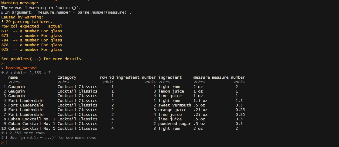
boston_parsed

boston_df <- 
  boston_parsed |> 
  select(-row_id, -ingredient_number, -measure) |> 
  pivot_wider(names_from = ingredient,values_from = measure_number, 
              values_fill = 0) |> 
  clean_names() |> 
  na.omit()

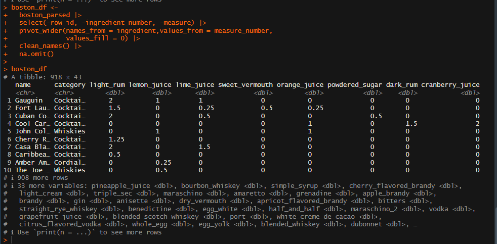
boston_df

pivot_wider() is used to put our data in a wider format and the clean_names() is a function from the lubridate package

boston_pca <- 
  boston_df |> 
  recipe( ~.) |> 
  update_role(name, category,new_role = "id") |> 
  step_normalize(all_predictors()) |> 
  step_pca(all_predictors())

prep_pca <- prep(boston_pca)

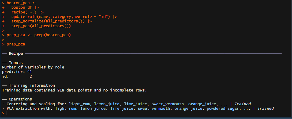
prep_pca

The recipe() function is from the recipe package and offers numerous data preprocessing functions and steps we used the step_normalize() to center and scale our data and use the the update_role() to tell our algorithm that the columns selected are nor required in the learning and should be used only for "id" which can be seen in the image below

tidied_pca <- tidy(prep_pca,2)

tidied_pca

The tidy() function from the tidyr package can be used to extract our Principal Components

tidied_pca |> 
  filter(component %in% paste0("PC", 1:5)) |> 
  mutate(component = fct_inorder(component)) |> 
  ggplot(aes(value,terms, fill = terms)) +
  geom_col(show.legend = FALSE) +
  facet_wrap(vars(component), nrow = 1) +
  labs(Y = NULL)

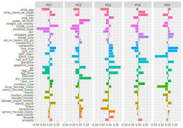
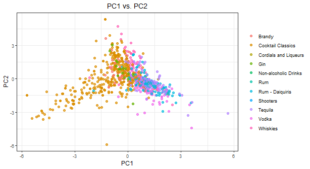
The final chart is showing the first 5 Principal Components and as stated earlier, the first 2 Principal Components i.e. PC1 and PC2 has more variance and explains more than 90% of the data dimensions