Machine learning (ML) is transforming industries by providing systems the ability to automatically learn and improve from experience without being explicitly programmed. This guide will introduce key concepts and techniques that form the backbone of machine learning, with a focus on regression and classification methods.

I. Introduction to Machine Learning

Machine learning is a subset of artificial intelligence (AI) that focuses on building systems capable of learning from data. At its core, ML is about finding patterns in data to make predictions or decisions. The primary types of machine learning are:

Supervised Learning: Learning from labeled data to predict outcomes.
Unsupervised Learning: Finding hidden patterns in unlabeled data.

Reinforcement Learning: Learning by interacting with an environment to achieve goals.

II. Linear Regression

Linear Regression is the most basic algorithm in Machine Learning. It is a regression algorithm which means that it is useful when we are required to predict continuous values A few examples of the regression problem include-

“What is the market value of the house?”
“Stock price prediction”
“Sales of a shop”
“Predicting height of a person”

Terms to be used here:

Features — These are the independent variables in any dataset represented by x1 , x2 , x3, x4,… xn for ’n’ features.
Target / Output Variable — This is the dependent variable whose value depends the independent variable by a relation (given below) and is represented by ‘y’.
Function or Hypothesis of Linear Regression is represented by — y = m1 x1 + m2 x2 + m3 x3 + … + mn xn + b

Note: Hypothesis is a function that tries to fit the data.
Intercept — Here b is the intercept of the line. So modified form of above equation is as follows: y = mx Where mx = m1.x1 + m2.x2 + m3.x3 + … + mn.xn + mn+1.xn+1 Here mn+1 is b and xn+1 = 1
Training Data — This data contains a set of dependent variables that is ‘x’ and a set of output variable, ‘y’.

Linear Regression with one variable or feature:

To understand Linear Regression better and visualize the graphs, let us assume that there is only one feature in the dataset, that is, x. So the equation goes as follows:

Y = mX + b

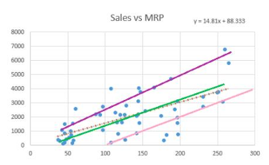
Let’s say if we scatter the points (x,y) from our training data, then what linear regression tries to do is, it tries to find a line with (given m and b ) such that error of each data point (x,yactual) is minimum when compared with x, ypredicted. Error here means combined error. This line is also called line of best fit .

Look at the graph given below :

Here it is difficult to find out the line of best fit just by looking at the different lines.There can be three ways of calculating error function:

Sum of residuals (∑(Yactual — Ypredict)) — it might result in cancelling out of positive and negative errors.
Sum of the absolute value of residuals (∑ | Yactual — Ypredict | ) — absolute value would prevent cancellation of errors.

3. Sum of square of residuals ( ∑ ( Yactual — Ypredict )²) — it’s the method mostly used in practice since here we penalize higher error value much more as compared to a smaller one, so that there is a significant difference between making big errors and small errors, which makes it easy to differentiate and select the best fit line.

III. Multivariable Regression

Multivariable regression extends linear regression to include multiple independent variables, enabling the model to capture more complex relationships.

Equation:
y=β0+β1x1+β2x2+…+βnxn+ϵ

IV. Gradient Descent

Gradient Descent

Optimization is a big part of machine learning. Almost every machine learning algorithm has an optimization algorithm at its core.
Gradient descent is an optimization algorithm used to find the values of parameters (coefficients) of a function (f) that minimizes a cost function (cost).\

Procedure:

Let the cost function be, f:

The procedure starts by assuming the initial values of coefficients. These could be 0.0 or some random value.

Coefficient, m = 0 Intercept, b = 0

The cost is evaluated by using these coefficients.

Cost = f (m, b)

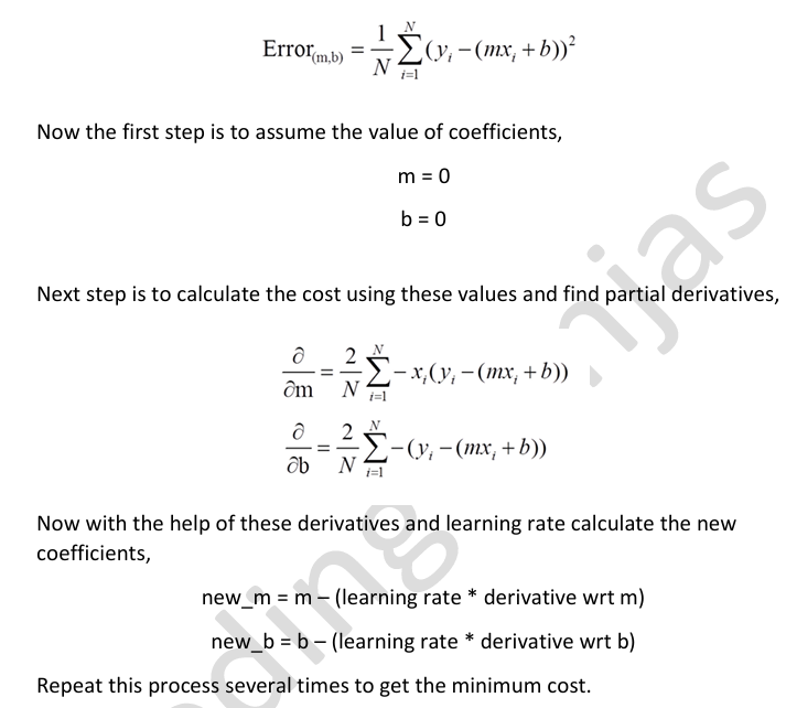
Now derivative of cost is calculated with respect to the coefficients i.e. slope of the cost function is calculated. We need to know the slope to determine the direction to move the coefficient values to get lower cost at next iteration.

Delta = derivative(cost), i.e.

Now to update the coefficient values, a learning rate parameter must be specified on each iteration

New-coefficients = coefficient — (learning-rate*derivative)

Repeating this process enough times will give the coefficients that will result in minimum cost.

Example, in case of Linear Regression with only one feature, cost function is given as:

V. Feature Scaling

Feature Scaling is a data preprocessing technique. By preprocessing, we mean the transformations that are applied to the data before it is fed into some algorithm for some processing.
Feature scaling or re-scaling of the features is performed such that they have the properties of normal distribution (most of the time) where values have standard deviation = 1, and mean = 0.

How Feature Scaling is applied in sklearn?

There are many ways by which we can apply feature scaling on the dataset:

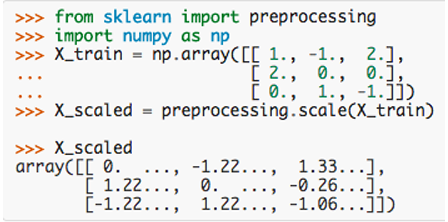
1. The easiest way of scaling is to use — preprocessing.scale() function A numpy array of values is given as input and output is numpy array with scaled values.

This will scale the values in such a way that mean of the values will be 0 and standard deviation will be 1.

3. Another method is to scale the features between given minimum and maximum values, generally between 0 and 1.

Function -preprocessing.MinMaxScaler(feature_range=(0, 1), copy=True) Feature_range is given in the form of tuple — (min , max) Copy — True (default), set it to False if you want inplace transformation

Formula used -

VI. Logistic Regression

Logistic Regression

Logistic regression is used for binary classification, predicting the probability of an instance belonging to one of two classes.

Key Concepts

Binary Outcomes: Suitable for tasks with two possible outcomes, like spam detection (spam or not spam).
Logistic Function: Uses the sigmoid function to map predicted values to probabilities between 0 and 1:

Log-Odds: Models the log-odds of the probability, where the log-odds is the logarithm of the odds ratio.

Applications

Spam Detection: Classifies emails as spam or not spam.
Medical Diagnosis: Predicts disease presence based on patient data.
Credit Scoring: Assesses the likelihood of loan default.

Advantages

Simple and Interpretable: Easy to understand and implement.
Efficient: Less computationally intensive than complex models.

Limitations

Linearity Assumption: Assumes a linear relationship between features and log-odds.
Sensitive to Imbalanced Data: Performance may degrade with imbalanced classes.

Logistic regression is a powerful tool for binary classification, offering simplicity and interpretability, making it a popular choice for many applications.

VII. Classification Measures

Classification measures are metrics used to evaluate the performance of classification models

Confusion Matrix

A confusion matrix is a table used to evaluate the performance of a classification model. It provides a detailed breakdown of correct and incorrect predictions.

Structure of a Confusion Matrix

For a binary classification problem, the confusion matrix is a 2x2 table consisting of:

Key Metrics Derived from the Confusion Matrix

Accuracy: The proportion of total correct predictions.

Precision: The ratio of true positive predictions to the total predicted positives. Measures the accuracy of positive predictions.

Recall (Sensitivity): The ratio of true positive predictions to the actual positives. Measures the ability of the model to capture positive instances

F1 Score: The harmonic mean of precision and recall, providing a balance between the two metrics.

Specificity: The ratio of true negative predictions to the actual negatives. Measures the model’s ability to identify negative instances.

VIII. Conclusion

Machine learning, through its core regression and classification techniques, provides powerful tools for solving diverse problems across industries. Understanding concepts like linear and logistic regression, along with evaluation metrics such as precision and recall, equips beginners to tackle both continuous and categorical data challenges.

Machine Learning Basics: Simple Guide to Regression and Classification for Beginners