Imagine a world where you can train high-performing machine learning models without the tedious and expensive task of manually labeling vast amounts of data.

How do you decide which data points to label?

This is the promise of active learning.

Active learning transforms the traditional approach to model training by strategically selecting the most informative data points for labeling.

By doing so, it significantly reduces the labeling effort while maintaining or even improving model performance.

What is Active Learning?

Active learning is an intelligent data labeling strategy that enables ML to achieve high performance with minimal human supervision.

It iteratively selects the most informative samples from a pool of unlabeled data for labeling.That helps to maximize model performance with minimal labeled data.

Unlike traditional supervised learning, where you label a large dataset upfront, active learning focuses on labeling only the most valuable data points.

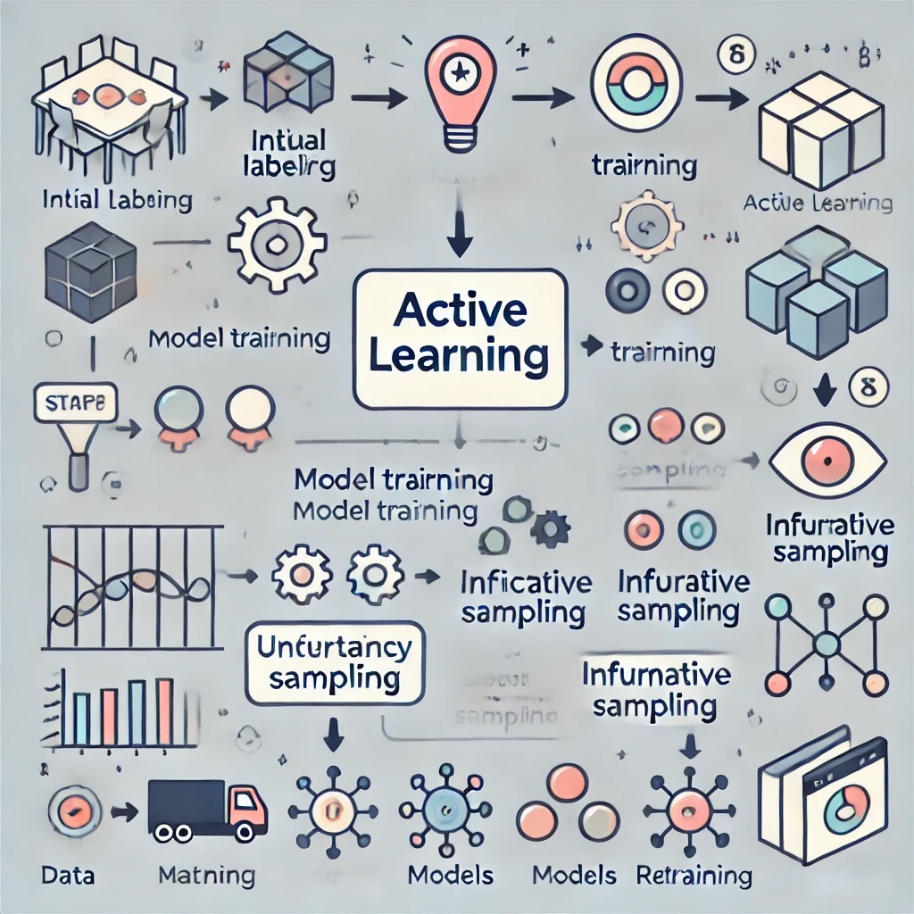
The Active Learning Cycle

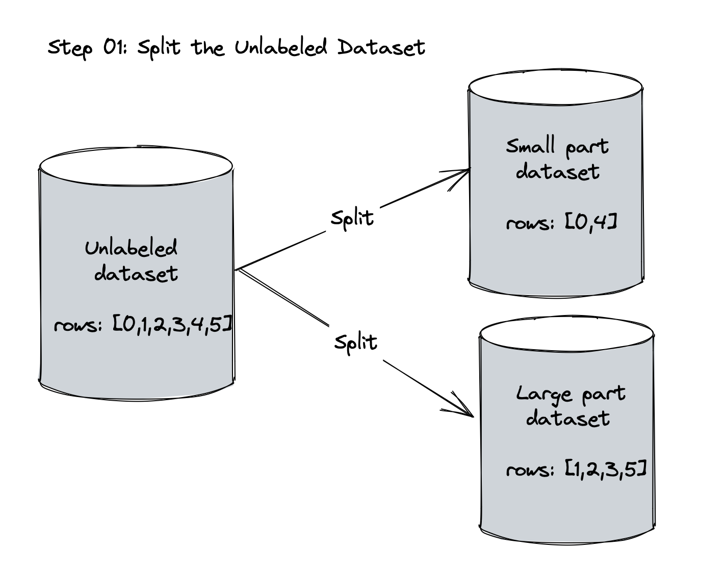
Split the dataset into small and large set, and label the small set
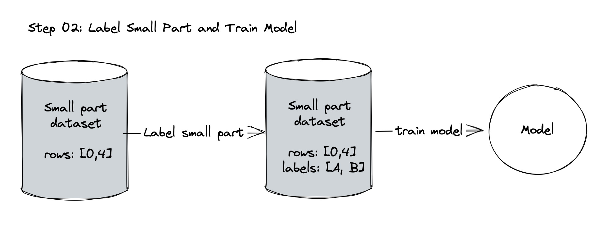
Train an initial model on the labeled small set.
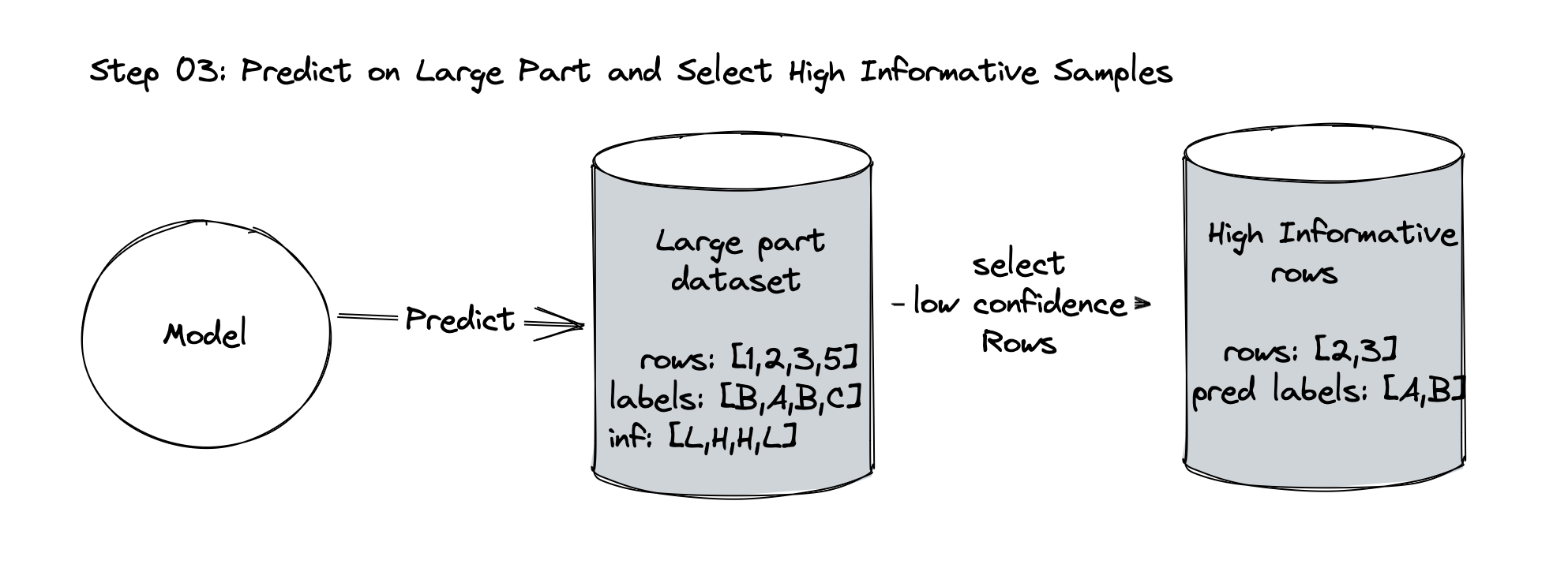
Use the model to make predictions on the unlabeled large set.
Select the most informative unlabeled samples based on certain criteria.
Label these selected samples.
Add the newly labeled samples to the small set.
Retrain the model and repeat the process.

Why Active Learning?

The primary advantage of active learning is efficiency. Labeling data is often costly and time-consuming.

Active learning helps by reducing the amount of data that needs manual labeling.

This technique enables models to achieve high performance with fewer labeled samples, saving both time and resources.

Consider these scenarios where active learning shines:

Medical image classification where expert radiologists are needed for labeling
Sentiment analysis of customer reviews where manual annotation is required
Speech recognition systems that need transcribed audio data
Autonomous vehicles that require labeled sensor data for object detection

Strategies for Selecting Informative Samples

Selecting the most informative samples is critical for the success of active learning.

Let's explore some key strategies:

Uncertainty Sampling

Uncertainty sampling is perhaps the most intuitive and widely used approach in active learning.

It focuses on selecting samples where the model is least certain about its predictions.

Several methods measure uncertainty:

Least Confidence Method

This method selects samples with the lowest predicted probability for the most likely class.

import numpy as np

def least_confidence_sampling(model, unlabeled_data, n_samples):
    probabilities = model.predict_proba(unlabeled_data)
    uncertainty = 1 - np.max(probabilities, axis=1)
    selected_indices = np.argsort(uncertainty)[-n_samples:]
    return selected_indices

Margin Sampling

Margin sampling looks at the difference between the two highest class probabilities.

A small margin indicates that the model is having difficulty distinguishing between the top two classes.

def margin_sampling(model, unlabeled_data, n_samples):
    probabilities = model.predict_proba(unlabeled_data)
    sorted_probs = np.sort(probabilities, axis=1)
    margins = sorted_probs[:, -1] - sorted_probs[:, -2]
    selected_indices = np.argsort(margins)[:n_samples]
    return selected_indices

Entropy-Based Sampling

Entropy is a measure of uncertainty in information theory.

In the context of active learning, we select samples with the highest entropy in their predicted class probabilities.

def entropy_sampling(model, unlabeled_data, n_samples):
    probabilities = model.predict_proba(unlabeled_data)
    entropies = -np.sum(probabilities * \
        np.log(probabilities + 1e-10), axis=1)
    selected_indices = np.argsort(entropies)[-n_samples:]
    return selected_indices

Query by Committee (QBC) Method

Query by Committee is an ensemble-based approach to active learning.

The idea is to train multiple models (a committee) and select samples where the models disagree the most.

This disagreement can be measured in various ways:

Vote Entropy

Vote entropy measures the disagreement among committee members based on their predicted classes.

def vote_entropy_sampling(models, unlabeled_data, n_samples):
    predictions = np.array(
        [model.predict(unlabeled_data) for model in models]
    )
    vote_counts = np.apply_along_axis(lambda x: \
        np.bincount(x, minlength=len(models[0].classes_)), \
        axis=0, arr=predictions)
    vote_proportions = vote_counts / len(models)
    entropies = -np.sum(vote_proportions * \
        np.log(vote_proportions + 1e-10), axis=1)
    selected_indices = np.argsort(entropies)[-n_samples:]
    return selected_indices

Kullback-Leibler (KL) Divergence

KL divergence measures the difference between probability distributions predicted by different models.

from scipy.stats import entropy

def kl_divergence_sampling(models, unlabeled_data, n_samples):
    probabilities = np.array(
        [model.predict_proba(unlabeled_data) for model in models]
    )
    avg_prob = np.mean(probabilities, axis=0)
    kl_divs = np.array(
        [entropy(avg_prob.T, prob.T) for prob in probabilities]
    )
    mean_kl = np.mean(kl_divs, axis=0)
    selected_indices = np.argsort(mean_kl)[-n_samples:]
    return selected_indices

Diversity Sampling Method

While uncertainty and disagreement are important, we also want to ensure that we're exploring diverse regions of the feature space.

Diversity sampling aims to select a set of samples that are representative of the entire unlabeled pool.

Clustering-Based Sampling

One approach to diversity sampling is to use clustering algorithms to group similar samples and select representatives from each cluster.

from sklearn.cluster import KMeans

def diversity_sampling(unlabeled_data, n_samples):
    kmeans = KMeans(n_clusters=n_samples)
    kmeans.fit(unlabeled_data)
    selected_indices = []
    for cluster_center in kmeans.cluster_centers_:
        closest_index = np.argmin(
            np.linalg.norm(unlabeled_data - cluster_center, axis=1)
        )
        selected_indices.append(closest_index)
    return selected_indices

Hybrid Approaches Method

In practice, combining different strategies often yields the best results.

For example, we might use uncertainty sampling to identify a pool of uncertain samples, then apply diversity sampling to ensure we're covering different regions of the feature space.

def hybrid_sampling(
    model, unlabeled_data, n_samples, uncertainty_ratio=0.7
):
    n_uncertainty = int(n_samples * uncertainty_ratio)
    n_diversity = n_samples - n_uncertainty

    # Uncertainty sampling
    uncertainty_indices = least_confidence_sampling(
        model, unlabeled_data, n_uncertainty
    )

    # Diversity sampling on the remaining data
    remaining_data = np.delete(
        unlabeled_data, uncertainty_indices, axis=0
    )
    diversity_indices = diversity_sampling(remaining_data, n_diversity)

    # Combine the selected indices
    selected_indices = np.concatenate(
        [uncertainty_indices, diversity_indices]
    )
    return selected_indices

Challenges and Considerations in Active Learning

While active learning offers significant benefits, it's not without its challenges:

Selection Bias

The criteria for selecting informative samples must be carefully designed to avoid introducing bias.

Biased sample selection can lead to skewed models that do not generalize well to unseen data.

Computational Cost

Active learning involves training multiple models iteratively, which can be computationally expensive.

Balancing the computational cost with the benefits of reduced labeling effort is crucial.

Human in the Loop

Active learning often requires human annotators to label the selected samples.

Ensuring consistent and accurate labeling is essential for the success of the active learning process.

Real-World Applications of Active Learning

Active learning has found success in various domains where labeled data is scarce or expensive to obtain:

Medical Image Analysis

In medical imaging, expert radiologists are often needed to label images, making the labeling process time-consuming and expensive.

Active learning can significantly reduce the number of images that need expert annotation.

For example, in a study on brain tumor segmentation, active learning achieved comparable performance to full supervision while using only 50% of the labeled data.

Autonomous Vehicles

Self-driving cars generate vast amounts of sensor data that need to be labeled for object detection and scene understanding.

Active learning helps focus the labeling effort on the most informative frames, reducing the overall annotation workload.

Cybersecurity

Active learning is used in intrusion detection systems to adaptively select network traffic patterns for expert analysis, improving the system's ability to detect new types of attacks.

Conclusion

Active learning represents a paradigm shift in how we approach machine learning with limited labeled data.

By intelligently selecting the most informative samples for labeling, it allows us to build high-performance models with minimal human annotation effort.

This not only saves time and resources but also opens up new possibilities in domains where labeled data is scarce or expensive to obtain.

As we've explored in this article, active learning is not a one-size-fits-all solution.

It requires careful consideration of selection strategies, implementation details, and domain-specific challenges.

However, when implemented effectively, it can dramatically accelerate the development of machine learning models and enable applications that were previously impractical due to data limitations.

Unlocking the Power of Active Learning: A Deep Dive into Smart Data Labeling