Understanding Linear Regression in Machine Learning
 Utkal Kumar Das
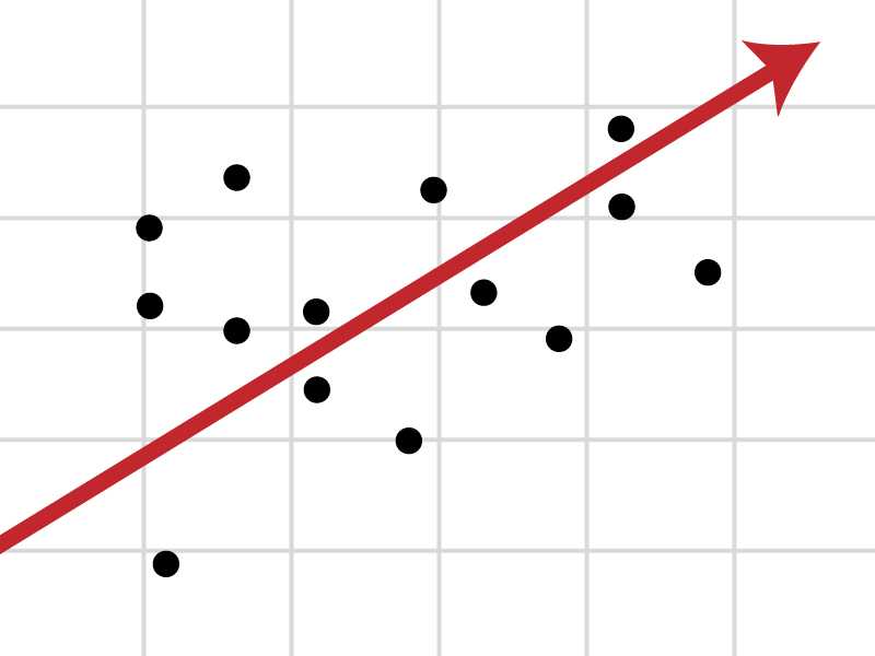
Regression in ML is a supervised learning algorithm which computes a relationship between dependent and independent variables.
It is most often used to predict an output from multiple possible outputs. (in most of the cases it is a number)
There are two types of regressions we use in machine learning. They are-
Linear Regression
Logistic Regression
In this blog, we'll learn about basics of Linear regression and implement it in python.
Linear Regression
Linear regression is a type of supervised-machine learning algorithm which computes a linear relationship between a dependable variable and other independent variables.
Linear regression is of two types -
Simple Linear Regression - It involves only one dependent variable and one independent variable.
Multiple Linear Regression - It involve one dependent variable and more than one independent variables
Simple Linear Regression
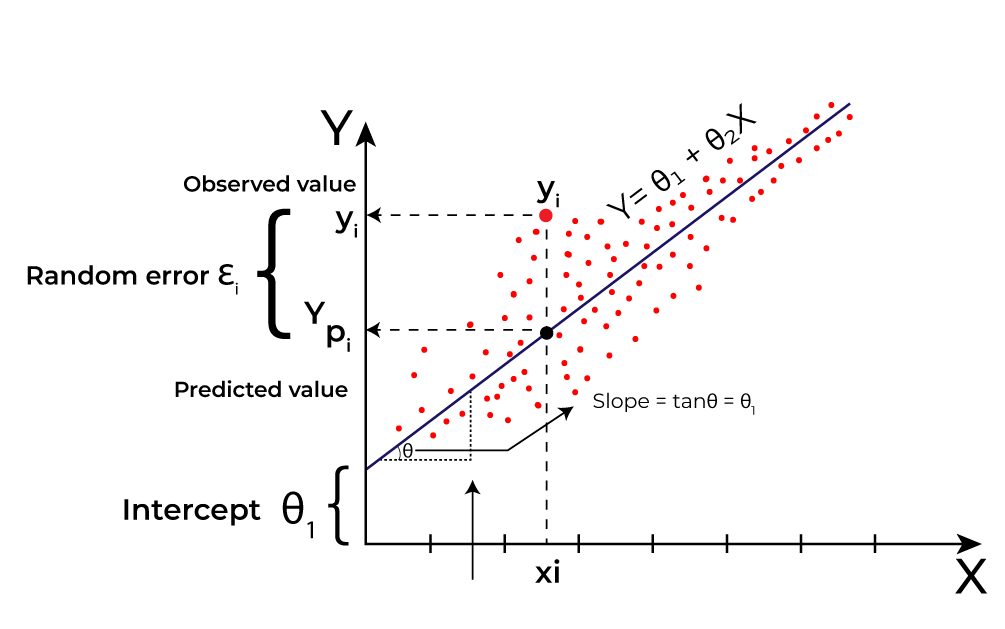
A simple linear regression computes a relationship between one dependent variable and one independent variable. It is represented by -
$$\hat{y} = w.x + b$$
where:
\(\hat{y}\) is the dependent variable (output)
\(x\) is the independent variable (input)
\(w\) is the slope
\(b\) is the intercept
** \(y\) and \(\hat{y}\) are two different terms, where:
\(y\) is the true value (used to train the model)
\(\hat{y}\) is the output value obtained from the linear regression model
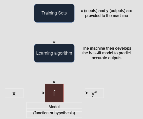
The goal of a simple linear regression algorithm is to find the best-fit Line equation between the inputs and outputs. As the name suggests 'best-fit Line', it implies that the error between the predicted values and actual values should be minimum.
Here, Y is the output variable and X is the input variable.
Linear regression is a model that performs the task to predict the output \(\hat{y}\) based on the given input \(x\).
Predicting the values of \(w\) and \(b\)
In order to achieve the equation (of best-fit line) that predicts the output value (\(\hat{y}\)), such that the error between the predicted values (\(\hat{y}\)) and the true value (\(y\)) is minimum, we need to update the values of \(w\) and \(b\).
Cost Function
Cost Function is nothing but an error calculator between the predicted values (\(\hat{y}\)) and the true values (\(y\)).
In Linear regression, we use Mean Squared Error (MSE) cost function to calculate the average of the squared error between the predicted values (\(\hat{y}_i\)) and true values (\(y_i\)). The purpose of the cost function is to determine the values of \(w\) and \(b\) that would minimize the error of the linear regression model.
The MSE cost function can be calculated as:
$$J(w,b) = \frac{1}{2m}\times\sum_{i=1}^m(\hat{y}_i-y_i)^2$$
where:
\(J(w,b)\) represents the cost function.
\(m\) is the total number of training sets.
\(i = (1, 2, 3,.... m)\)
The graph of \(J(w,b)\) or cost function is bowl shaped.
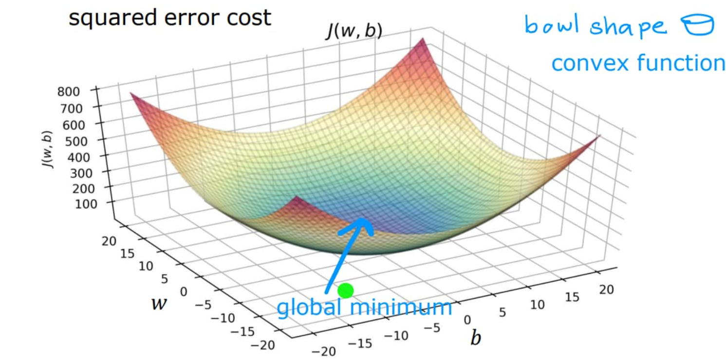
So, the values of \(w\) and \(b\) for which \(J(w,b)\) will be minimum is the best-fit for the Linear regression model.
Gradient Descent
Gradient descent is just an optimization algorithm used to train Linear regression model to reduce the cost function to the minimum by modifying the parameters \(w\) and \(b\) iteratively. The idea is to start with random values of \(w\) and \(b\) and then iteratively update the values to reach minimum \(J(w,b)\).
The algorithm of Gradient descent:
repeat till convergence {
\(w = w - \alpha\frac{\partial}{\partial w}J(w,b)\)
\(b = b - \alpha\frac{\partial}{\partial b}J(w,b)\)
}
Differentiating \(J\) with respect to \(w\) :
\(\frac{\partial}{\partial w}J(w,b)\)
\(= \frac{\partial}{\partial w}\sum_{i=1}^m\frac{1}{2m}(\hat{y}_i-y_i)^2\)
\(= \frac{1}{2m}\frac{\partial}{\partial w}\sum_{i=1}^m((w\times x_i + b)-y_i)^2\)
\(= \frac{1}{m}\sum_{i=1}^m(\hat{y}_i-y_i).x_i\)
Differentiating \(J\) with respect to \(b\) :
\(\frac{\partial}{\partial b}J(w,b)\)
\(= \frac{\partial}{\partial b}\sum_{i=1}^m\frac{1}{2m}(\hat{y}_i-y_i)^2\)
\(= \frac{1}{2m}\frac{\partial}{\partial b}\sum_{i=1}^m((w\times x_i + b)-y_i)^2\)
\(= \frac{1}{m}\sum_{i=1}^m(\hat{y}_i-y_i)\)
The Gradient descent algorithm (after putting the values of partial derivatives):
repeat till convergence{
\(w = w - \alpha\frac{1}{m}\sum_{i=1}^m(\hat{y}_i-y_i).x_i\)
\(b = b - \alpha\frac{1}{m}\sum_{i=1}^m(\hat{y}_i-y_i)\)
}
where:
\(w\) and \(b\) are the parameters of linear regression model
\(\alpha\) is the learning rate
Learning Rate (\(\alpha\)) -
Learning rate (\(\alpha\)) is a constant multiplied to the partial derivative term which determines how fast we reach minimum \(J(w,b)\).
If \(\alpha\) is too small, then the gradient descent may be slow and it would take a long time to reach minimum \(J(w,b)\).
If \(\alpha \) is too large, then the gradient descent may overshoot and never reach minimum \(J(w,b)\).
Therefore, we should choose a learning rate (\(\alpha\)) that's neither too small nor too large.

So, this is it for the mathematics part of Linear regression, now let's go through the python implementation of Linear regression model.
Python Implementation of Linear regression model
To understand the Linear regression model, we are going to use basic python with some frameworks such as numpy and matplotlib here.
Let's take a small dataset and develop a Linear regression model for it.
| Size (in 1000 sq ft.) | Price (in 1000s of dollars) |
| 1.0 | 300 |
| 1.5 | 360 |
| 2.0 | 500 |
| 2.75 | 540 |
| 3.0 | 650 |
First, we will import all the necessary libraries.
import math, copy
import numpy as np
import matplotlib.pyplot as plt
Entering the data and storing them in an array which will be used to train the linear regression model.
x_train = np.array([1.0, 1.5, 2.0, 2.75, 3.0])
y_train = np.array([300.0, 360.0, 500.0, 540.0, 650.0,])
m = x_train.shape[0] #total number of training datasets
Now, computing the Linear regression model by taking some random values of parameters \(w\) and \(b\).
w = 100
b = 100

def compute_model_output(x, w, b):
  m = x.shape[0]
  y_hat = np.zeros(m)
  for i in range(m):
    y_hat[i] = w*x[i] + b   #predicted values
  return y_hat

temp_y_hat = compute_model_output(x_train, w, b)
Let's plot the graph and see how fit is our Linear regression model.
plt.plot(x_train, temp_y_hat, c='b', label="our predictions")
plt.scatter(x_train, y_train, marker='x', c='r')
plt.title("Housing prices")
plt.ylabel("Price (in 1000s of dollars)")
plt.xlabel("Size (in 1000 sqft.)")
plt.show()
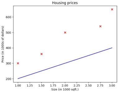
It's clearly visible that it is not the best fit Linear regression model for our dataset. We need to update the values of the parameters \(w\) and \(b\).
Now we'll calculate the MSE Cost function to find the error between the predicted and true values.
def compute_cost(x, y, w, b):
  m = x.shape[0]
  cost_sum = 0
  for i in range(m):
    y_hat = w*x[i] + b
    cost = (y_hat - y[i])**2
    cost_sum += cost
  total_cost = cost_sum / (2*m)
  return total_cost

a = compute_cost(x_train, y_train, w, b)
print(a)
$$15182.5$$
The value of cost function is too high, we need to run the Gradient descent algorithm to update the values of \(w\) and \(b\) to minimize cost function.
Let's now write the code for Gradient descent algorithm (which is the main objective of Linear regression).
# computing gradient (partial derivative)
def compute_gradient(x, y, w, b):
  m = x.shape[0]
  dj_dw = 0
  dj_db = 0
  for i in range(m):
    y_hat = w*x[i] + b
    dj_dw_i = (y_hat - y[i])*x[i]
    dj_db_i = (y_hat - y[i])
    dj_dw += dj_dw_i
    dj_db += dj_db_i
  dj_dw = dj_dw / m
  dj_db = dj_db / m
  return dj_dw, dj_db
def gradient_descent(x, y, w_in, b_in, alpha, num_iters, cost_function, gradient_function):
  # x = input data
  # y = target values
  # w_in and b_in = initial values of w and b
  # alpha = learning rate
  # num_iters = number of iterations to run gradient descent
  # cost_function = function to compute cost
  # gradient_function = function to compute gradient

  J_history = [] # history of cost values
  p_history = [] # history of parameters w and b
  w = w_in
  b = b_in

  for i in range(num_iters):
    dj_dw, dj_db = gradient_function(x, y, w, b)
    w = w - (alpha * dj_dw)
    b = b - (alpha * dj_db)

    # Save cost J at each iteration
    if (i < 100000): # to prevent resource exhaustion
      J_history.append(cost_function(x, y, w, b))
      p_history.append([w,b])
    # Print cost at every 10 intervals and at every interval if i<10
    if (i % math.ceil(num_iters/10) == 0):
            print(f"Iteration {i:4}: Cost {J_history[-1]:0.2e} ",
                  f"dj_dw: {dj_dw: 0.3e}, dj_db: {dj_db: 0.3e}  ",
                  f"w: {w: 0.3e}, b:{b: 0.5e}")
  return w, b, J_history, p_history

iterations = 10000
tmp_alpha = 0.01
w_final, b_final, J_hist, p_hist = gradient_descent(x_train ,y_train, w, b, tmp_alpha, iterations, compute_cost, compute_gradient)
print(f"(w,b) found by gradient descent: ({w_final:8.4f},{b_final:8.4f})")

Now, we got the best-fit values of parameters \(w\) and \(b\), by which we can achieve the most optimized Linear regression model for the given dataset.
Let's plot the graph again after obtaining the values of parameters \(w\) and \(b\).
temp_y_hat = compute_model_output(x_train, w_final, b_final)

plt.plot(x_train, temp_y_hat, c='b', label="our predictions")
plt.scatter(x_train, y_train, marker='x', c='r')
plt.title("Housing prices")
plt.ylabel("Price (in 1000s of dollars)")
plt.xlabel("Size (in 1000 sqft.)")
plt.show()
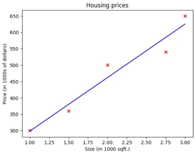
So, now we got the best-fit line, which means we have successfully trained the Linear regression model for our dataset. We can now enter new test values (size in 1000 sqft.) and the model will give us the output (price in 1000s of dollars) with minimum error.
x_test = np.array([2.75])
y_hat_test = compute_model_output(x_test, w_final, b_final)
print(f"The predicted price for a house of size {x_test[0]*1000} sqft. is ${round(y_hat_test[0]*1000,2)}")

Multiple Linear Regression
A multiple linear regression computes a relationship between one dependent variable and more than one independent variable. It is represented by -
$$\hat{y} = \vec{w}.\vec{x} + b$$
where:
\(\hat{y}\) is the dependent variable (output)
\(\vec{x}\) is the vector of all the independent variables (inputs)
\(\vec{w}\) is a vector of parameters corresponding to each \(x\)
(the value of each \(w\) corresponding to the \(x\) (feature) depends on how much it affects the output result)
\(b\) is another parameter
To understand Multiple linear regression, we can take help of the previous example of prediction of Housing price, where there was only one independent variable (\(x\)) (size of the housing) and one dependent variable (\(\hat{y}\)) (price). But we know that the Price of the house depends on a lot of factors other than size, like age of the house, location and more.
So, to predict the price of the house more accurately we have to consider more than one independent variables like age and size together to build a Linear regression model.
The method to train a Multiple linear regression model is mostly same as that of Simple linear regression model except for in place of all the scaler calculations, we use vector calculations. Later, in the upcoming blogs I'll discuss more about Multiple Linear regression.
Conclusion
So, this was quite everything about Linear Regression in Machine Learning. After reading this blog, you should now have a basic understanding of Linear Regression and be able to implement it in Python.
If you have any questions or need further clarification on any of the topics discussed, feel free to leave a comment below or reach out to me directly. Let's learn and grow together!
LinkedIn: https://www.linkedin.com/in/utkal-kumar-das-785074289
To further explore the world of machine learning, here are some recommended resources:
Coursera: Machine Learning by Andrew Ng-https://www.coursera.org/learn/machine-learning
Towards Data Science- https://towardsdatascience.com/
Subscribe to my newsletter
Read articles from Utkal Kumar Das directly inside your inbox. Subscribe to the newsletter, and don't miss out.
Written by

Utkal Kumar Das
Utkal Kumar Das
🤖 Machine Learning Enthusiast | 🌐 aspiring Web Developer 🔍 Currently Learning Machine Learning 🚀 Future plans? Eyes set on mastering Competitive Programming, bagging internships, winning competitions, and crafting meaningful projects.
