Remember that hilarious scene from Silicon Valley where Jian-Yang tried to pitch a "Shazam for food" app that could only identify hotdogs? Well, I took that ridiculous idea and made it a reality! Here's how I created a working app using a simple neural network trained on a custom-made dataset, and why it's more than just a joke.

All the code used in this article can be found on my Github.

Creating a ML model

Import necessary libraries

To train our ML model, I'll be using PyTorch because it gives us a lot of control over what we want to implement. First, we need to import a few necessary libraries. You can find the list of required modules here.

import os
import glob
import shutil
import torch 
from tqdm import tqdm
import torch.nn as nn
from torchvision import transforms,datasets,models
from torch.nn.modules.loss import BCEWithLogitsLoss
from torch.optim import lr_scheduler
import numpy as np 
import matplotlib.pyplot as plt

#use GPU if available
device = torch.device("cuda" if torch.cuda.is_available() else "cpu")

Quest for the Perfect Hotdog

You might think that finding a dataset of hotdog images would be a piece of cake (or should I say, a slice of bun?). Initially, I explored several datasets on Kaggle, but the accuracy of the model trained on these datasets was disappointingly low.

The main issue was the low number of images for classifying hotdogs, compared to the large number of images showing what is 'not' a hotdog.

So, I did what any dedicated developer would do: I rolled up my sleeves and created a custom dataset. This involved countless hours of scouring the internet for hotdog pictures and meticulously labeling them. I ensured that the images for each class were equal in number to reduce the model bias.

The result? A mouthwatering dataset now available on Kaggle for others to use. And it make a difference! My model's accuracy jumped by about 10% compared to my previous attempts.

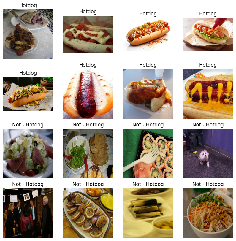
Here's a glimpse of the dataset looks:

#select random samples from the dataset
samples_hotdog = [os.path.join(hotdog_train,np.random.choice(os.listdir("/train/hotdog"),1)[0]) for _ in range(8)]
samples_others = [os.path.join(others_train,np.random.choice(os.listdir("/train/others"),1)[0]) for _ in range(8)]

nrows = 4
ncols = 4

fig, ax = plt.subplots(nrows,ncols,figsize = (10,10))
ax = ax.flatten()

for i in range(nrows*ncols):
  if i < 8:
    pic = plt.imread(samples_hotdog[i%8])
    ax[i].imshow(pic)
    ax[i].set_axis_off()
    ax[i].set_title('Hotdog')
  else:
    pic = plt.imread(samples_others[i%8])
    ax[i].imshow(pic)
    ax[i].set_axis_off()
    ax[i].set_title('Not - Hotdog')
plt.show()

Running the above code returns a result like this:

Those look delicious! The next step is to do some data pre-processing to feed these images to our neural network.

Art of Image Transformations

Before feeding our images into the neural network, we need to prepare them. This is where image transformation comes into play, and it's a crucial step in any computer vision task. Let's see why it's important and how do we implement it in our workflow:

• Consistency: Neural networks expect input data to be uniform. Resizing all images to a specific resolution ensures that our model receives consistent input, regardless of the original image dimensions.

• Normalization: Normalizing pixel values helps our model converge faster during training. This process involves scaling the pixel values to a standard range, typically between 0 and 1, or to have a mean of 0 and a standard deviation of 1.

• Performance Optimization: Properly preprocessed images can lead to faster training times and improved model performance

traindir = "/train"
testdir = "/test"
validdir="/val"

#transformations
img_transforms = transforms.Compose([transforms.Resize((224,224)),
                                       transforms.ToTensor(),                                
                                       torchvision.transforms.Normalize(
                                           mean=[0.485, 0.456, 0.406],
                                           std=[0.229, 0.224, 0.225],)])

#datasets
train_data = datasets.ImageFolder(traindir,transform=img_transforms)
test_data = datasets.ImageFolder(testdir,transform=img_transforms)
valid_data= datasets.ImageFolder(validdir,transform=img_transforms)

#dataloader
trainloader = torch.utils.data.DataLoader(train_data, shuffle = True, batch_size=16)
testloader = torch.utils.data.DataLoader(test_data, shuffle = True, batch_size=16)
validloader= torch.utils.data.DataLoader(test_data, shuffle = True, batch_size=16)

Let's break down what's happening here:

1. Resizing: We use transforms.Resize((224,224)) to ensure all images are the same size. This is crucial because our model expects inputs of this specific dimension.

2. Tensor Conversion: transforms.ToTensor() converts the image from a PIL Image or numpy.ndarray to a torch.FloatTensor. It also scales the image's pixel values to the range [0.0, 1.0]. In PyTorch data needs to be represented in the form of a torch.Tensor(). You can read more about it here.

3. Normalization: We use torchvision.transforms.Normalize() with specific mean and standard deviation values. These values ([0.485, 0.456, 0.406] for mean and [0.229, 0.224, 0.225] for std) are the standard normalization values for models pre-trained on ImageNet, which includes our model.

4. Composition: transforms.Compose() allows us to chain these transformations together, applying them in sequence to our images.

We then apply these transformations to our training, testing, and validation datasets using PyTorch's ImageFolder class. This class automatically labels images based on the folder structure of our dataset.

Finally, we create DataLoader objects for each dataset. These are incredibly useful as they handle batching data, shuffling it for training, and loading it in parallel using multiple workers.

The Power of transfer Learning

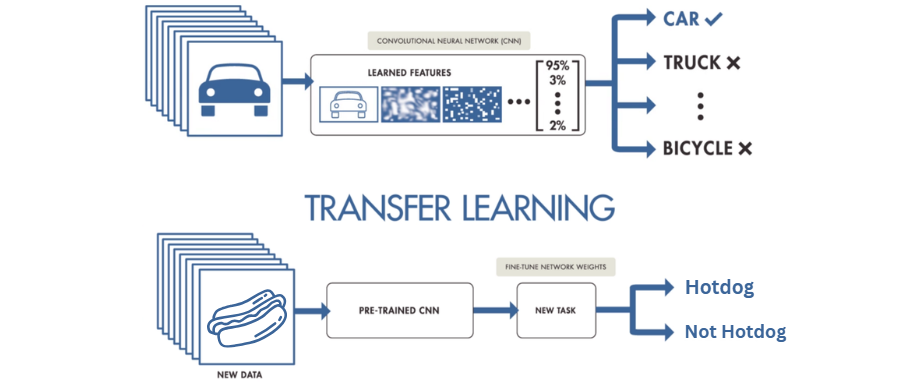
At the heart of this project lies the magic of transfer learning. For those unfamiliar with the concept, transfer learning is a technique in machine learning where we take a pre-trained neural network (usually trained on a massive dataset) and use it as a starting point for a new, more specific task.

In my case, I chose the ResNet18 model as the foundation and modified the final layer for binary classification. ResNet18 is a convolutional neural network pre-trained on ImageNet, a dataset of over a million images across 1000 categories. The beauty of transfer learning is that we don't have to start from scratch. Instead, we fine-tune the existing model by adjusting its weights to fit our specific problem.

We can implement this concept in PyTorch as follows:

model = models.resnet18(pretrained=True)

#freeze all params
for params in model.parameters():
  params.requires_grad_ = False

#add a new final layer
nr_filters = model.fc.in_features  #number of input features of last layer
model.fc = nn.Linear(nr_filters, 1)

model = model.to(device)

Creating the training loop

Now that we've prepared our data and set up our model, it's time for the main event: training our neural network to distinguish hotdogs from not-hotdogs. At its core, a training loop is a repetitive process where we:

1. Feed batches of images through our model.

2. Compare the model's predictions to the actual labels.

3. Calculate the loss (how wrong our model is).

4. Use backpropagation to compute gradients.

5. Update the model's weights to improve its performance.

def make_train_step(model, optimizer, loss_fn):
  def train_step(x,y):
    #make prediction
    yhat = model(x)
    #enter train mode
    model.train()
    #compute loss
    optimizer.zero_grad()
    loss = loss_fn(yhat,y)
    loss.backward()
    optimizer.step()
    return loss
  return train_step

#loss function
loss_fn = BCEWithLogitsLoss() 
#optimizer
optimizer = torch.optim.Adam(model.fc.parameters()) 
#train step
train_step = make_train_step(model, optimizer, loss_fn)

losses = []
val_losses = []
epoch_train_losses = []
epoch_test_losses = []

n_epochs = 15

for epoch in range(n_epochs):
  epoch_loss = 0
  for i ,data in tqdm(enumerate(trainloader), total = len(trainloader)): #iterate ove batches
    x_batch , y_batch = data
    x_batch = x_batch.to(device) #move to gpu
    y_batch = y_batch.unsqueeze(1).float() #convert target to same nn output shape
    y_batch = y_batch.to(device) #move to gpu
    loss = train_step(x_batch, y_batch)
    epoch_loss += loss/len(trainloader)
    losses.append(loss)
  epoch_train_losses.append(epoch_loss)
  print('\nEpoch : {}, train loss : {}'.format(epoch+1,epoch_loss))
  #validation doesnt requires gradient
  with torch.no_grad():
    cum_loss = 0
    for x_batch, y_batch in testloader:
      x_batch = x_batch.to(device)
      y_batch = y_batch.unsqueeze(1).float() #convert target to same nn output shape
      y_batch = y_batch.to(device)
      #model to eval mode
      model.eval()

      yhat = model(x_batch)
      val_loss = loss_fn(yhat,y_batch)
      cum_loss += loss/len(testloader)
      val_losses.append(val_loss.item())

    epoch_test_losses.append(cum_loss)
    print('Epoch : {}, val loss : {}'.format(epoch+1,cum_loss))  

# saving the model as a .pt file
torch.save(model,"/detection.pt")

Checking the predictions

Before we deploy our model, we need to check if it is giving us correct predictions. We check this using our validation data.

#making Predictions
def inference(valid_data):
  idx = torch.randint(1, len(valid_data), (1,))
  sample = torch.unsqueeze(valid_data[idx][0], dim=0).to(device)

  if torch.sigmoid(model(sample)) < 0.5:
    print("Prediction : Hot Dog")
  else:
    print("Prediction : Not a Hot Dog")
  plt.imshow(test_data[idx][0].permute(1, 2, 0))
inference(valid_data)

This will return a random image from our validation dataset with the model's prediction.

Deploying our model

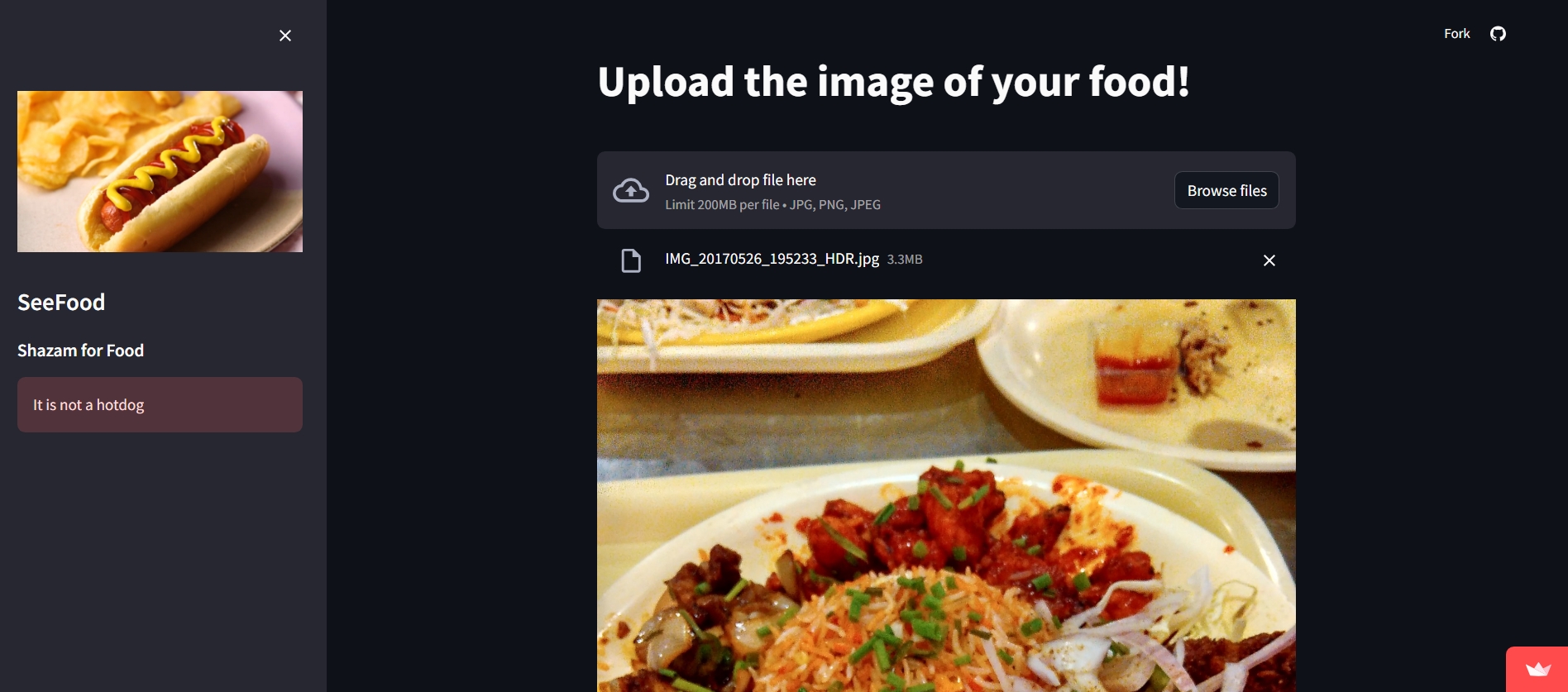
We Deploy our model as a user-friendly web app using a library called Streamlit. It is a popular framework for creating interactive web applications.

#create a file named app.py
import streamlit as st  
import torch 
from PIL import Image, ImageOps
import numpy as np

# hide deprication warnings which directly don't affect the working of the application
import warnings
warnings.filterwarnings("ignore")
# set some pre-defined configurations for the page, such as the page title, logo-icon, page loading state (whether the page is loaded automatically or you need to perform some action for loading)
st.set_page_config(
    page_title="SeeFood",
    page_icon = ":pizza:",
    initial_sidebar_state = 'auto'
)
def load_model():
    model=torch.load('detection.pt', map_location=torch.device('cpu'))
    model.eval()
    return model
with st.spinner('Model is being loaded..'):
    model=load_model()
# hide the part of the code, as this is just for adding some custom CSS styling but not a part of the main idea 
hide_streamlit_style = """
    <style>
  #MainMenu {visibility: hidden;}
    footer {visibility: hidden;}
  </style>
"""
st.markdown(hide_streamlit_style, unsafe_allow_html=True) # hide the CSS code from the screen as they are embedded in markdown text. Also, allow streamlit to unsafely process as HTML
with st.sidebar:
        st.image('dog.jpg')
        st.title("SeeFood")
        st.subheader("Shazam for Food")
st.write("""
         # Upload the image of your food!
         """
         )
file = st.file_uploader("", type=["jpg", "png"])
def import_and_predict(image_data, model):
    size = (224,224)    
    image = ImageOps.fit(image_data, size, Image.LANCZOS)
    img = np.asarray(image)
    img = img / 255
    img = torch.from_numpy(img).float().unsqueeze(0)
    img = img.permute(0, 3, 1, 2) 
    prediction = torch.sigmoid(model(img))
    return prediction.detach().numpy()

if file is None:
    st.text("Please upload theimage of the food you would like to know about.")
else:
    image = Image.open(file)
    st.image(image, use_column_width=True)
    predictions = import_and_predict(image, model)
    if predictions[0]<0.5:
        st.balloons()
        st.sidebar.success("It's a hotdog !!")
    else:
        st.sidebar.error("It is not a hotdog")

While our app might seem like a silly project (and let's be honest, it kind of is), it demonstrates some powerful concepts in machine learning and computer vision. Transfer learning, custom dataset creation, and deploying models as web applications are all valuable skills in AI development.