Time & Space Complexity

Time and space complexity can be measured in similar ways. In this article I'm focusing on time complexity, but the main difference between time and space complexity is how time increases and how much space is used, meaning how much data is stored in variables. Therefore, understanding one will help you understand both.

O(1)

The size of the input or data doesn’t affect operation time. For example:

• Inserting or removing at the end of an array(list), or getting an element from a specific index in the array.

    nums = [1, 2, 3, 4]   # Array
    nums.append(5)        # push to end
    nums.pop()            # pop from end
    nums[0]               # lookup
  

• Or inserting or removing a value from HashMap(dictionary) or HashSet(sets), or inserting a key or looking for some specific value.

    hashmap = {}             # HashMap / Set
    hashmap['key'] = 10      # insert
    print('key' in hashmap)  # lookup
    print(hashmap['key'])    # lookup
    hashmap.pop('key')       # remove
  

O(n)

The size of input affects processing time, in a linear fashion. For example:

• Inserting or removing from the start or middle of a list as every element needs to be shifted by 1 position.

    nums = [1, 2, 3, 4, 5]
    nums.insert(1, 100)  # insert middle
    nums.remove(100)     # remove middle
    print(100 in nums)   # search
  

• Summing the array or looping through the array under the hood.

    sum(nums)        # sum of array
    for n in nums:   # looping
       print(n)
  

• Heapifying a set of values i.e., building a heap out of an array.

    import heapq
    heapq.heapify(nums)   # build heap
  

• Sometimes even nested loops can be O(n) e.g., sliding window or monotonic stack algorithm.

  Checkout neetcode.io

O(n²)

The processing time is twice as compared to the size of the input. For example:

• Iterating through a 2D array.

• Iterating through a 1D array twice.

  • In a way that the full array is iterated in a nested loop.

      nums_list = [[1, 2], [3, 4]]
    
      # traversing a square grid
      for nums in nums_list:
         for num in nums:
            print(num)
    

  • Or the inner loop keeps decreasing the array size by 1. In this case, the time complexity is $n^2/2$, but as we don’t consider constants the time complexity becomes O(n²).

      nums = [1, 2, 3, 4, 5]
    
      # get every pair of elements in the array
      for num1 in nums:
         for num2 in nums[i+1:]:
            print(num1, num2)
    

• Insertion sort as it inserts in the middle of the array n-times.

O(m*n)

The processing time is the cross-product of the input sizes.

For example:

• Using nested loops to loop through two different size arrays.

    nums1, nums2 = [1, 2, 3], [4, 5]
  
    # get every pair of elements from 2 arrays
    for num1 in nums1:
       for num2 in nums2:
          print(num1, num2)
  

• Traversing through a rectangular grid.

    nums = [[1, 2, 3], [4, 5, 6]]
  
    # traversing the rectangular grid
    for nums in nums_list:
       for num in nums:
          print(num)
  

O(logn)

On every iteration of loop, we eliminate half of a loop.

For example:

• Binary Search

• Binary Search on Binary Search tree

• Heap push and pop

O(nlogn)

It has a better processing time than O(n) but a worse processing time than O(logn).

For example:

• Merge sort algorithm

• Most built-in sorting functions have O(nlogn) time complexity

• Heapsort, as if we have a heap of length n and we use heappop() to remove elements form it, then n times performing logn operation means nlogn.

    import heapq
  
    nums = [1, 2, 3, 4, 5]
    heapq.heapify(nums)   # O(n)
    # heapsort
    while nums:           # loop through n elements
        heapq.heappop(nums) # O(logn)
  

O(2^n)

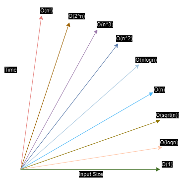
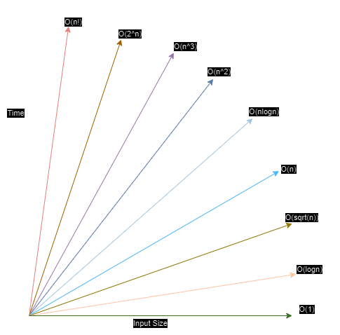
This is a non-polynomial run time. This equation is just a reflection O(nlogn) over the diagonal axis (orange line in the image).

For example,

• Recursion

    # recursion, tree height n, two branches, i.
    def recursion(i, nums):
        if i == len(nums):
            return 0
        branch1 = recursion(i + 1, nums)
        branch2 = recursion(i + 2, nums)
  

O(√n)

It is pretty rare in coding interviews. It is also a non-polynomial run time.

Example,

• Getting all factors of a constant.

    import math
    n = 12
    factors = set()
    for i in range(1, int(math.sqrt(n)) + 1):
        if n % i == 0:
            factors.add(i)
            factors.add(n // i)
    print(factors)
  

O(n!)

It is pretty rare, it may come in,

• permutation problem, or

• graph problem like travelling salesman problem.

It is very inefficient, so if your solution is n! then you don’t have the optimal solution but sometimes n! is the best you can do.

Reference:

Diagram

Reference: Big-O Notation - Full Course