Activating Activation Functions

If the neural network is alive, it will think what is its purpose here or what is its goal in the world. The main goal of any neural network is to transform the non-linearly separable input data into more linearly separable abstract features using a hierarchy of layers. In these hierarchy of layers, they contain functions that enable the network to learn complex pattens, control information flow and make accurate predictions. So, with the help of activation functions, neural networks can effectively tackle a wide range of problems, from simple linear regression to complex tasks. They determine whether a neuron should be activated or not.

Activation function is a mathematical formula that performs the transformation of a vector available in a binary, float or integer format to another format based on the type of mathematical transformation function. In neural networks, we have three kinds of layers — input, hidden and output and these layers are interconnected through a mathematical function called an activation function. The importance of activation function in a neural network can be known from following purposes:

1. Introducing non-linearity: it should add non-linearity in the optimization landscape to improve the convergence in training of network.

2. Controlling the information flow: They help in regulating the information flow by deciding which data is relevant and which is not.

3. Decrease complexity: It should not increase the computational complexity of model extensively.

4. Handling complex data: They allow complex data and make accurate predictions retaining data distribution to facilitate better training of the network.

A thought again arrives that all functions are activation functions. This though drives to the criteria for a function to be an activation function. There are several criteria, some important ones are:

1. Non-linearity: To enable the network to learn and model complex, non-linear relationships in the data.

2. Differentiability: To allow the use of gradient-based optimization methods like back-propagation.

3. Bounded Output: To prevent the output values from growing too large, which can help in stabilizing the learning process.

4. Computational Efficiency: To ensure that the function can be computed quickly and efficiently, which is crucial for training large networks.

5. Monotonicity: To ensure that the function is either non-decreasing or non-increasing which can help in simplifying the optimization process.

All activation functions that are part of a neural network model can be broadly classified as linear functions and nonlinear functions.

• Linear Activation functions: Simple, useful for linear relationships, but limited in modeling complexity.

• Non-Linear Activation Functions: Essential for capturing complex patterns, enabling the network to learn and represent intricate data relationships.

Let us know about different types of activation functions.

Import important libraries first.

import numpy as np
import torch
import torch.nn as nn
from torch.autograd import Variable
import torch.nn.functional as F
import matplotlib.pyplot as plt

Linear Function

A linear function is a simple function used to transfer information from demapping layer to the output layer. In the linear function, the output is always confined to a specific range because of which it is used in last hidden layer or in linear regression based tasks or in a deep learning where the task is to predict the outcome from the input dataset. The following is the formula:

x = Variable(torch.randn(100, 10))
y = Variable(torch.randn(100, 30))
linear = nn.Linear(in_features=10, out_features=5, bias=True)
output_linear = linear(x)
print('Output size: ', output_linear.size())
# Output size:  torch.Size([100, 5])

Bilinear Function

A bilinear function is a simple functions typically used to transfer information applying a bilinear transformation to incoming data.

bilinear = nn.Bilinear(in1_features=10, in2_features=30, out_features=5, bias=True)
output_bilinear = bilinear(x, y)
print('Output size: ', output_bilinear.size())
#Output size:  torch.Size([100, 5])

Sigmoid Function

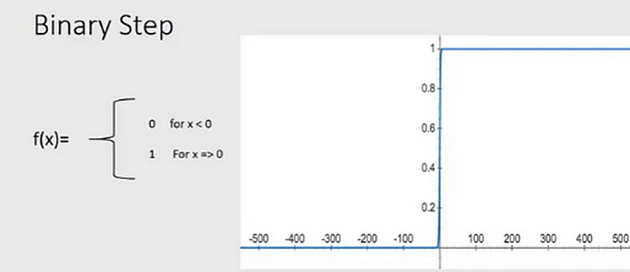
In mathematics, you must have seen a function.

Can you observe something? I have a condition that x must be greater than or equal to 0, in that case, the function gives true or 1. Otherwise, it gives false or 0. Still can’t think, we will go on a journey in upcoming article. Let’s focus on sigmoid and other activation functions.

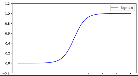
A sigmoid function is a nonlinear function to that lets our model to capture all sorts of nonlinearity present in data. It is always confined within 0 and 1. It is mostly used to perform classification tasks. One of the main limitations of the sigmoid function is that it may get stuck in local minima. An advantage is that it provides probability of belonging to the class. The following is its equation

x = Variable(torch.randn(100, 10))
y = Variable(torch.randn(100, 30))
sig = nn.Sigmoid()
output_sig = sig(x)
output_sigy = sig(y)
print('Output size: ', output_sig.size())
print('Output size: ', output_sigy.size())

Hyperbolic Tangent Function

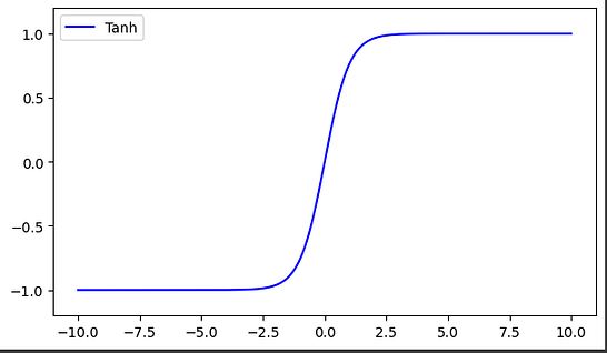
This is an another variant of transformation function. It is used to transform information from mapping layer to the hidden layer. It is typically used between the hidden layers of a neural network model. The range of tanh functions is between -1 and +1.

x = Variable(torch.randn(100, 10))
y = Variable(torch.randn(100, 30))
func = nn.Tanh()
output_x = func(x)
output_y = func(y)
print('Output size: ', output_x.size())
print('Output size: ', output_y.size())

Log Sigmoid Transfer Function

In large numeric values dataset in the input feature, we have lot of outliers of float type and data is not binary in this case then we can use log sigmoid transfer function.

x = Variable(torch.randn(100, 10))
y = Variable(torch.randn(100, 30))
func = nn.LogSigmoid()
output_x = func(x)
output_y = func(y)
print('Output size: ', output_x.size())
print('Output size: ', output_y.size())

ReLU Function

We have heard this name many times but it is rectified linear unit (ReLU) which is another activation function that is used in transferring information by firing the neurons from input layer to the output layer. It is mostly used between different hidden layers in a neural network model and its range is from 0 to infinity. There are different stages when this function can be used that is to go from input to the hidden layer and while going from hidden to output layer.

x = Variable(torch.randn(100, 10))
y = Variable(torch.randn(100, 30))
func = nn.ReLU()
output_x = func(x)
output_y = func(y)
print('Output size: ', output_x.size())
print('Output size: ', output_y.size())

Leaky ReLU

Now there are many problems arise in the neural network. One such problem of vanishing gradient has given birth to this activation function. Actually more better is to dying gradient problem and to avoid this issue, leaky ReLU is applied. Leaky ReLU allows a small and non-zero gradient when the unit is not active to make it active.

x = Variable(torch.randn(100, 10))
y = Variable(torch.randn(100, 30))
func = nn.LeakyReLU()
output_x = func(x)
output_y = func(y)
print('Output size: ', output_x.size())
print('Output size: ', output_y.size())

Visualisation of Activation Functions

Every function can be plotted by knowing their data range. They are nothing but curves in the graph or better I say space whether 2D or d-dimensional.

The activation functions translate the data from one layer to another layer. The transformed data can be plotted against the actual tensor to visualize the function.

Here we converted the vector to a Torch variable and then made a copy as a NumPy variable for plotting the graph.

x = torch.linspace(-10, 10, 1500)
x = Variable(x)
x_l = x.data.numpy()
y_relu = F.relu(x).data.numpy()
y_sigmoid = torch.sigmoid(x).data.numpy()
y_tanh = torch.tanh(x).data.numpy()
y_softplus = F.softplus(x).data.numpy()

plt.figure(figsize=(7, 4))
plt.plot(x_l, y_relu, c='blue', label='ReLU')
plt.ylim((-1, 11))
plt.legend(loc='best')

plt.figure(figsize=(7, 4))
plt.plot(x_l, y_sigmoid, c='blue', label='Sigmoid')
plt.ylim((-0.2, 1.2))
plt.legend(loc='best')

plt.figure(figsize=(7, 4))
plt.plot(x_l, y_tanh, c='blue', label='Tanh')
plt.ylim((-1.2, 1.2))
plt.legend(loc='best')

plt.figure(figsize=(7, 4))
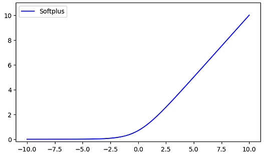
plt.plot(x_l, y_softplus, c='blue', label='Softplus')
plt.ylim((-0.2, 11))
plt.legend(loc='best')

This is all about the activation function in the neural network. Hope it will provide an insight to use activation function while preparing your model.

Thank you!

— Akhil Soni