How Convolutional Neural Networks (CNNs) Work: A Practical Guide with MNIST

Introduction

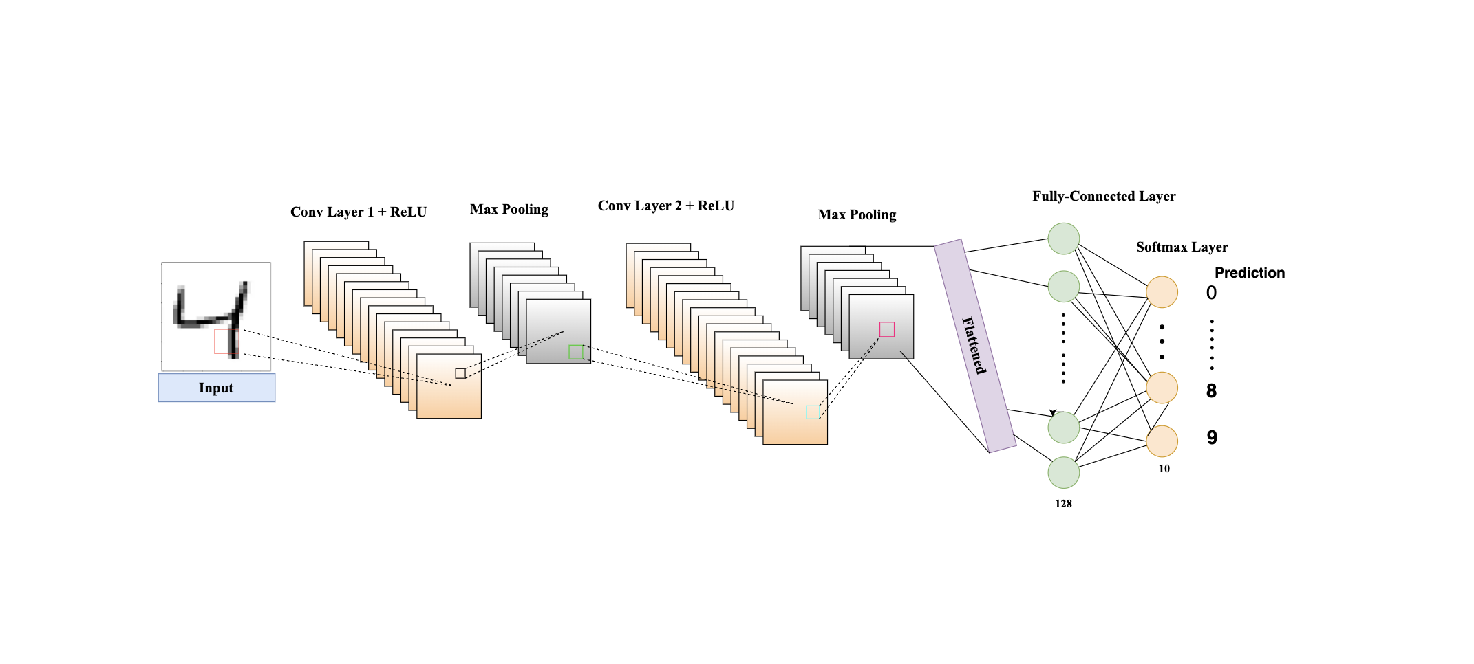
In the deep learning domain, one area that has really taken a revolutionary turn is that of Convolutional Neural Networks (CNNs) to enable machines to see images. What makes facial recognition, self-driving cars, and even medical image analysis so magical are the CNNs fueling them. This article explains CNNs and also demonstrates their application by building a handwritten digit recognizer using the MNIST dataset.

Understanding CNNs

Basic Concepts

CNNs are meant to work with image data. Their main components are:

Convolutional Layers: These are layers where a set of filters (kernels) is applied to the input image to develop the feature maps depicting aspects of the input, like edges and textures.

Pooling Layers: Reduces the spatial dimensions of feature maps with minimal loss of information.

Fully connected layers: These are the traditional neural network-like layers in which each neuron is connected to all the neurons in the previous layer, and the output features are used for making the final predictions.

How CNNs Work

1. Convolutional Layers

They are CNN's heart. This applies convolutional filters to input images in order to extract hierarchical features:

• Filters/Kernels: These small matrices (e.g., 3x3 or 5x5) slide across the image to identify specific features. Each filter is trained for different features, such as edges, textures, and patterns.

• Strides: This is the size of the steps a filter takes when it's moving through the image, in pixels. Larger strides reduce the output size and, therefore, the computational burden.

• Padding: Adding extra pixels at the image boundary so that its spatial dimensions are kept unchanged and no information is lost.

The convolution operation can be expressed as:

$$(I * K)(i, j) = \sum_m \sum_n I(i+m, j+n) \cdot K(m, n)$$

Where I is the input image, K is the filter, (i,j) and represents the position of the filter on the image.

Example: In the task of digit recognition, the early layers learn to detect edges or simple shapes, while deeper layers may learn to recognize a higher-order structure, such as curves or parts of digits.

2. Activation Functions

Activation functions bring nonlinearity to the network, which helps the network learn complex patterns.

• ReLU (Rectified Linear Unit): This is the most commonly used activation function. It will output the input directly when it is positive; otherwise, the output is zero:

  ReLU(x)=max⁡(0,x)

• Leaky ReLU: A variant of ReLU that allows a small, non-zero gradient when the input is negative:

  Leaky ReLU(x)=max(0.01⋅x,x)

• Sigmoid and Tanh: These are functions that squash the output to 0-1 and -1 to 1, respectively; thus, they are currently used less in modern CNNs.

Example: ReLU helps in training deep networks by mitigating the vanishing gradient problem, which can occur with functions like sigmoid.

3. Pooling Layers

The pooling layers reduce the spatial dimensions of feature maps, to make the model more computationally efficient and robust against variations.

• Max Pooling: This takes the maximum value from a group of neighbouring pixels:

  MaxPool(x)=(x_i,j)

• Average Pooling: This takes the average value from a group of neighbouring pixels.

Example: In digit recognition, pooling layers can reduce the size of feature maps while retaining the most important information, such as the overall shape of a digit.

4. Batch Normalization

Batch Normalization normalizes the activations of the network for speedy and stable training. It does this by adjusting the output from any layer to be of zero mean and unit variance:

$$\text{BN}(x) = \gamma \frac{x - \mu}{\sigma} + \beta$$

where:

• γ and 𝛽 are learnable parameters used to scale and shift the normalized output,

• 𝜇 is the mean of the batch,

• 𝜎 is the variance of the batch.

This normalization process helps keep the network's activations stable and makes training faster and more efficient by reducing changes in the distribution of the inputs across different layers.

5. Fully Connected Layers

Fully connected layers (or dense layers) interpret the features extracted by convolutional and pooling layers. They flatten the feature maps and make predictions:

• Flattening: Converts the 2D feature maps (i.e. 2D arrays) into a 1D vector (i.e. 1D array).

• Dense Layers: Each neuron in the dense layer is connected to every neuron in the previous layer, allowing the network to combine features and make decisions.

Example: In digit recognition, the fully connected layers combine high-level features extracted by the convolutional layers to classify the digit.

6. Regularization Techniques

To prevent overfitting, various regularization techniques can be used:

• Dropout: This technique randomly sets a fraction of the neurons to zero during training, forcing the network to learn redundant representations.

  $$\text{Dropout}(x) = \text{random_drop}(x)$$

• L2 Regularization: This technique adds a penalty proportional to the square of the weights to the loss function, discouraging overly complex models.

$$\text{Loss} = \text{Original Loss} + \lambda \sum_{i} w_{i}^{2}$$

Example: Dropout can ensure that the network does not overly rely on any single feature, leading to better generalization.

Practical Implementation: Handwritten Digit Recognition with MNIST

To see these concepts in action, let's implement a CNN for digit recognition using the MNIST dataset.

Loading and Preprocessing Data

import tensorflow as tf
import numpy as np
import matplotlib.pyplot as plt
from keras.datasets import mnist
import keras
from keras import layers

(x_train, y_train), (x_test, y_test) = mnist.load_data()

# Reshape and normalize the data
x_train = x_train.reshape(x_train.shape[0], 28, 28, 1).astype('float32') / 255
x_test = x_test.reshape(x_test.shape[0], 28, 28, 1).astype('float32') / 255

# Split training data into training and validation sets
from sklearn.model_selection import train_test_split
x_train, x_val, y_train, y_val = train_test_split(x_train, y_train, test_size=0.2, shuffle=True)

Building the CNN Model

We define a CNN model with multiple convolutional and pooling layers, followed by fully connected layers.

from keras.models import Model

input = keras.Input((x_train.shape[1], x_train.shape[2], 1))
conv2D = keras.layers.Conv2D(64, kernel_size=(3, 3), activation="relu", kernel_initializer='glorot_normal', name='ConvLayer1')(input)
conv2D = keras.layers.Conv2D(64, kernel_size=(3, 3), activation="relu", kernel_initializer='glorot_normal', name='ConvLayer2')(conv2D)
maxPool = keras.layers.MaxPool2D(pool_size=(2, 2), name='MaxPoolLayer1')(conv2D)
batchnorm = keras.layers.BatchNormalization()(maxPool)
conv2D = keras.layers.Conv2D(128, 3, activation='relu', kernel_initializer='glorot_normal', name='ConvLayer3')(batchnorm)
conv2D = keras.layers.Conv2D(128, 3, activation='relu', kernel_initializer='glorot_normal', name='ConvLayer4')(conv2D)
maxPool = keras.layers.MaxPool2D(pool_size=(2, 2), name='MaxPoolLayer2')(conv2D)
batchnorm = keras.layers.BatchNormalization()(maxPool)
flatten = keras.layers.Flatten()(batchnorm)
outputs = keras.layers.Dense(units=256, activation='relu')(flatten)
outputs = keras.layers.Dense(units=10, activation='softmax')(outputs)

model = Model(inputs=input, outputs=outputs)
model.compile(optimizer='adam', loss='sparse_categorical_crossentropy', metrics=['accuracy'])
model.summary()

Training and Evaluating the Model

history = model.fit(x_train, y_train, epochs=10, batch_size=128, validation_data=(x_val, y_val))

test_loss, test_accuracy = model.evaluate(x_test, y_test)
print(f"Test Accuracy: {test_accuracy}")

Extra Tip: Working with Custom Data

To test the model with your custom digit images, preprocess them as follows:

import cv2
import numpy as np
import math
from scipy import ndimage
import matplotlib.pyplot as plt

def preprocess_image(image_path):
    """
    Preprocess the input image for digit recognition.
    This involves converting to grayscale, resizing, inverting colors, 
    removing empty borders, and normalizing.
    """
    # Reading the image in grayscale
    gray = cv2.imread(image_path, cv2.IMREAD_GRAYSCALE)

    # Resizing the image to 28x28 and inverting the colors (black on white)
    gray = cv2.resize(255 - gray, (28, 28))
    _, gray = cv2.threshold(gray, 128, 255, cv2.THRESH_BINARY | cv2.THRESH_OTSU)

    # Removing empty borders to center the digit
    while np.sum(gray[0]) == 0:
        gray = gray[1:]

    while np.sum(gray[:, 0]) == 0:
        gray = np.delete(gray, 0, 1)

    while np.sum(gray[-1]) == 0:
        gray = gray[:-1]

    while np.sum(gray[:, -1]) == 0:
        gray = np.delete(gray, -1, 1)

    rows, cols = gray.shape

    # Resizing the image to maintain aspect ratio
    if rows > cols:
        factor = 20.0 / rows
        rows = 20
        cols = int(round(cols * factor))
        gray = cv2.resize(gray, (cols, rows))
    else:
        factor = 20.0 / cols
        cols = 20
        rows = int(round(rows * factor))
        gray = cv2.resize(gray, (cols, rows))

    # Padding the image to ensure it is 28x28
    cols_padding = (int(math.ceil((28 - cols) / 2.0)), int(math.floor((28 - cols) / 2.0)))
    rows_padding = (int(math.ceil((28 - rows) / 2.0)), int(math.floor((28 - rows) / 2.0)))
    gray = np.lib.pad(gray, (rows_padding, cols_padding), 'constant')

    return gray

def get_best_shift(img):
    """
    Calculate the shift required to center the image.
    """
    cy, cx = ndimage.center_of_mass(img)

    rows, cols = img.shape
    shiftx = np.round(cols / 2.0 - cx).astype(int)
    shifty = np.round(rows / 2.0 - cy).astype(int)

    return shiftx, shifty

def shift(img, sx, sy):
    """
    Shift the image by the specified amount.
    """
    rows, cols = img.shape
    M = np.float32([[1, 0, sx], [0, 1, sy]])
    shifted = cv2.warpAffine(img, M, (cols, rows))
    return shifted

# Defining image paths and their labels
image_paths_indices = [
    (2, '/content/drive/MyDrive/test digit/2.jpeg'),
    (3, '/content/drive/MyDrive/test digit/3.jpeg'),
    (4, '/content/drive/MyDrive/test digit/4.jpeg'),
    (7, '/content/drive/MyDrive/test digit/7.jpeg')
]

# Creating subplots for visualization
fig, axs = plt.subplots(2, 2, figsize=(8, 8))

for i, (original_digit, image_path) in enumerate(image_paths_indices):
    # Preprocess the image
    image_to_test = preprocess_image(image_path)

    # Optional: Center the digit in the image (commented out in this example)
    # shiftx, shifty = get_best_shift(image_to_test)
    # image_to_test = shift(image_to_test, shiftx, shifty)

    gray = image_to_test

    # Reshape the image for model prediction
    prediction_input = gray.reshape((-1, 28, 28, 1))

    # Predict the digit using the trained model
    prediction_probs = model.predict(prediction_input)
    predicted_digit = np.argmax(prediction_probs)

    # Display the image and predictions
    plt.subplot(2, 2, i + 1)
    plt.imshow(gray, cmap='gray')
    plt.text(0.5, -0.1, f'Original: {original_digit}\nPredicted: {predicted_digit}',
             horizontalalignment='center', verticalalignment='center', transform=plt.gca().transAxes)
    plt.axis('off')

plt.show()

Conclusion

Recently, the field of image processing and computer vision received a huge breakthrough with the inception of Convolutional Neural Networks. Deep learning models allowed researchers to reach the utmost accuracy in many tasks of interest, such as facial recognition, self-driving cars, or medical image analysis. In this article, we have gone through some basics of CNNs, such as convolutional layers, activation functions, pooling layers, batch normalization, and regularization techniques.

We explored how these concepts came together in implementing a CNN model for recognizing handwritten digits using the MNIST dataset, creating powerful tools for image classification. The practical example illustrates how effective CNNs are at pattern recognition and making accurate predictions.

CNNs are helpful in enabling advanced imaging applications and working on leading AI projects or just exploring the amazing world of deep learning. Fully mastering CNNs is key to unlocking the full potential of machine learning and artificial intelligence.