Predicting Loan Approval Risk: A Comprehensive Guide
 Debanjan Chakraborty
Table of contents

Introduction
Predicting loan approval risk is a critical task for financial institutions. Accurate predictions can help banks and lenders minimize risks and make informed decisions. In this blog post, we will explore a comprehensive approach to building and evaluating machine learning models to predict loan approval risk. We will use a dataset containing various features about loan applicants and train three different models: Decision Tree, Logistic Regression, and Neural Network. Additionally, we will analyze the bias and fairness of these models to ensure ethical and fair predictions.
First, we need to download the data
The data is available on my Kaggle page: https://www.kaggle.com/datasets/hydracsnova/loan-approval-dataset
Uploading and Loading the Dataset
First, let's upload and load our dataset into the Jupyter notebook.
# Upload file
from google.colab import files

uploaded = files.upload()

for fn in uploaded.keys():
  print('User uploaded file "{name}" with length {length} bytes'.format(
      name=fn, length=len(uploaded[fn])))
After uploading the dataset, we load it using pandas.
import pandas as pd
import matplotlib.pyplot as plt
import seaborn as sns
from sklearn.preprocessing import OneHotEncoder, StandardScaler
from sklearn.compose import ColumnTransformer
from sklearn.model_selection import train_test_split
from sklearn.tree import DecisionTreeClassifier, plot_tree
from sklearn.linear_model import LogisticRegression
from sklearn.metrics import classification_report, confusion_matrix, accuracy_score
from sklearn.utils.class_weight import compute_class_weight
from imblearn.over_sampling import SMOTE
import joblib
import tensorflow as tf
from tensorflow.keras.models import Sequential
from tensorflow.keras.layers import Dense

# Load the CSV file
data_file = '/content/loan_approval_dataset.csv'  # Change this to the path of your uploaded file
print("Loading data...")
data = pd.read_csv(data_file)
Data Preprocessing
We start by selecting the relevant columns for our analysis and then splitting the data into features (X) and the target variable (y).
selected_columns = ['Income', 'Age', 'Experience', 'Married_Single', 'House_Ownership', 'Car_Ownership', 'CURRENT_JOB_YRS', 'CURRENT_HOUSE_YRS', 'Risk_Flag']
data = data[selected_columns]

X = data.drop('Risk_Flag', axis=1)
y = data['Risk_Flag']
Next, we set up one-hot encoding for categorical columns and scale the numerical features.
print("Setting up categorical columns for one-hot encoding...")
categorical_columns = ['Married_Single', 'House_Ownership', 'Car_Ownership']
preprocessor = ColumnTransformer(
    transformers=[
        ('cat', OneHotEncoder(handle_unknown='ignore'), categorical_columns)
    ], remainder='passthrough')

print("Scaling numerical features...")
numerical_features = ['Income', 'Age', 'Experience', 'CURRENT_JOB_YRS', 'CURRENT_HOUSE_YRS']
scaler = StandardScaler()
X[numerical_features] = scaler.fit_transform(X[numerical_features])

print("Applying preprocessor...")
X_processed = preprocessor.fit_transform(X)
Handling Class Imbalance
Class imbalance is a common issue in datasets. We use the Synthetic Minority Over-sampling Technique (SMOTE) to handle this problem.
print("Applying SMOTE to handle class imbalance...")
smote = SMOTE(random_state=42)
X_resampled, y_resampled = smote.fit_resample(X_processed, y)
Splitting the Data
We split the data into training and testing sets.
print("Splitting data into training and testing sets...")
X_train, X_test, y_train, y_test = train_test_split(X_resampled, y_resampled, test_size=0.2, random_state=42)
Data Visualization
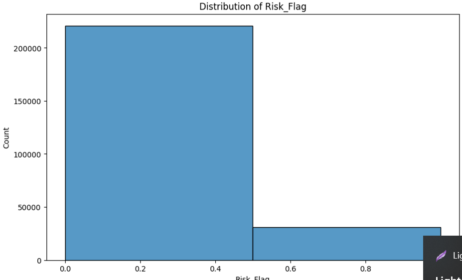
Data visualization helps in understanding the distribution and relationships within the dataset.
print("Visualizing data...")
plt.figure(figsize=(10, 6))
sns.histplot(y, bins=2, kde=False)
plt.title('Distribution of Risk_Flag')
plt.show()
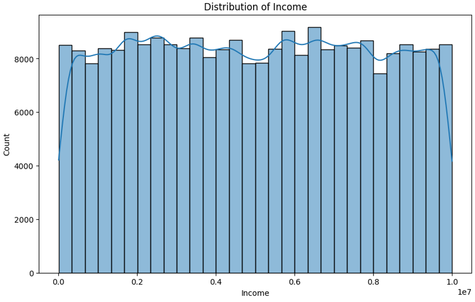
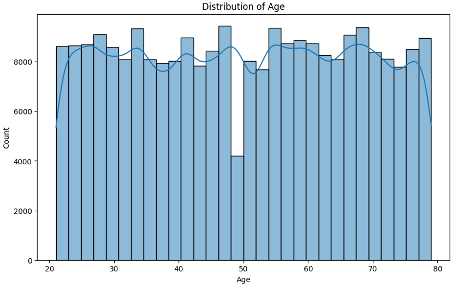
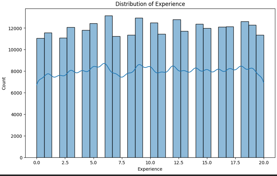
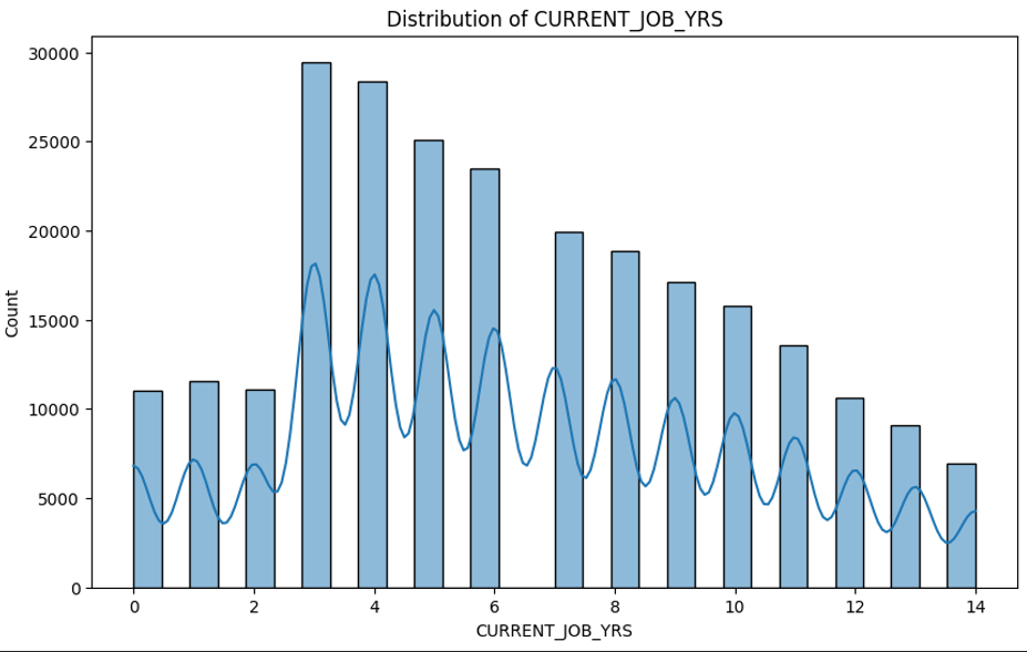
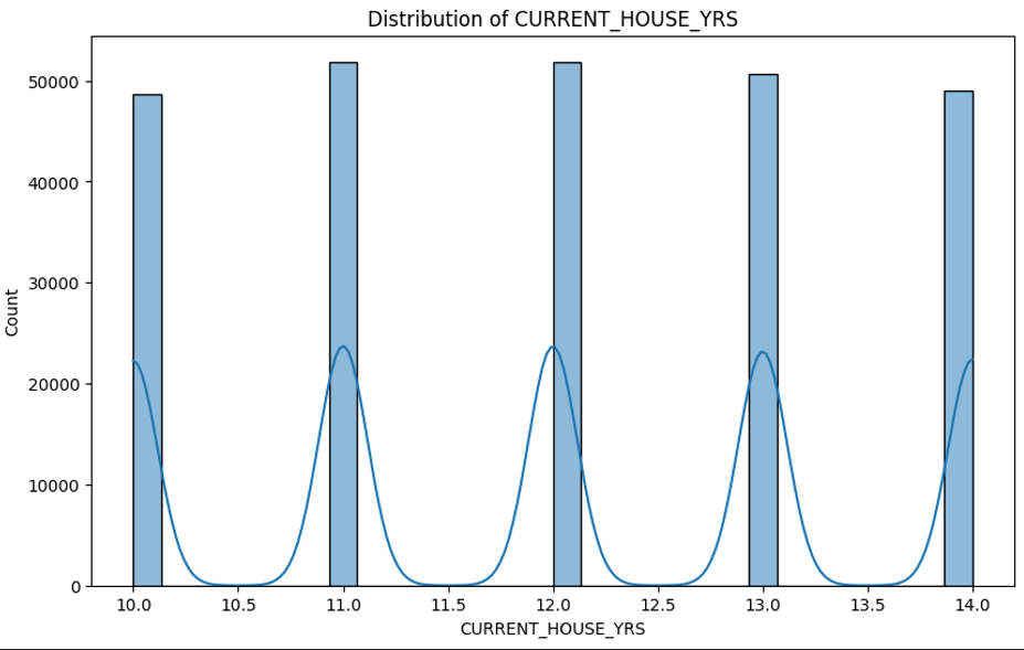
For numerical features:
for feature in numerical_features:
    plt.figure(figsize=(10, 6))
    sns.histplot(data[feature], bins=30, kde=True)
    plt.title(f'Distribution of {feature}')
    plt.show()
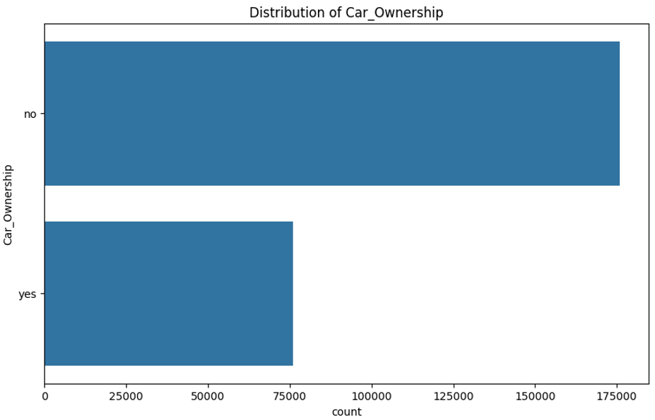
For categorical features:
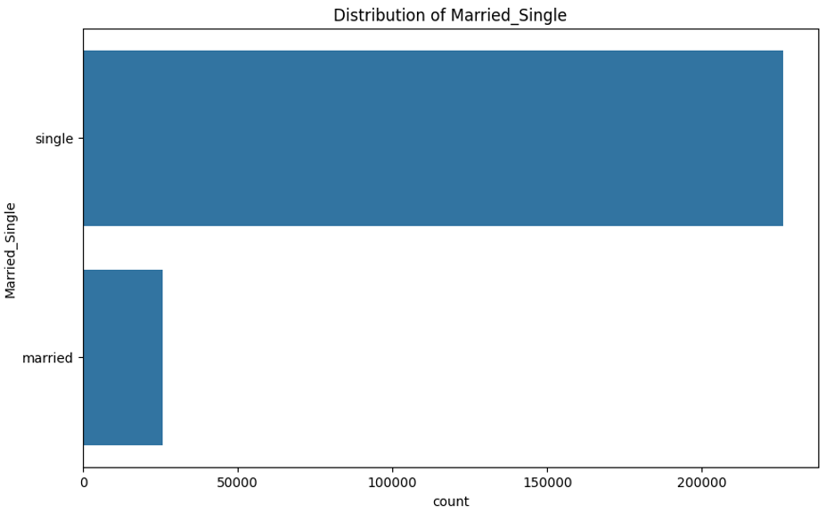
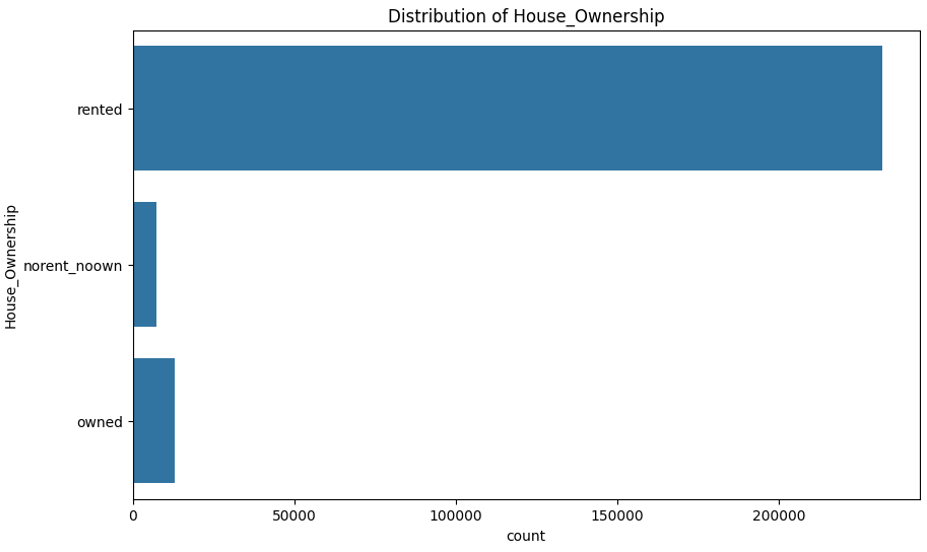
for feature in categorical_columns:
    plt.figure(figsize=(10, 6))
    sns.countplot(data[feature])
    plt.title(f'Distribution of {feature}')
    plt.show()
Training Models
Decision Tree Model
We start by training a decision tree model.
print("Training decision tree model...")
decision_tree_model = DecisionTreeClassifier(random_state=42)
decision_tree_model.fit(X_train, y_train)
Evaluate the model:
y_pred_train_tree = decision_tree_model.predict(X_train)
y_pred_test_tree = decision_tree_model.predict(X_test)

print("Decision Tree Training Set Evaluation:")
print(f"Accuracy: {accuracy_score(y_train, y_pred_train_tree)}")
print("Classification Report:")
print(classification_report(y_train, y_pred_train_tree))
print("Confusion Matrix:")
print(confusion_matrix(y_train, y_pred_train_tree))

print("\nDecision Tree Testing Set Evaluation:")
print(f"Accuracy: {accuracy_score(y_test, y_pred_test_tree)}")
print("Classification Report:")
print(classification_report(y_test, y_pred_test_tree))
print("Confusion Matrix:")
print(confusion_matrix(y_test, y_pred_test_tree))
Logistic Regression Model
Next, we train a logistic regression model.
print("Training logistic regression model...")
class_weights = compute_class_weight('balanced', classes=[0, 1], y=y_resampled)
logistic_model = LogisticRegression(max_iter=1000, random_state=42, class_weight={0: class_weights[0], 1: class_weights[1]})
logistic_model.fit(X_train, y_train)
Evaluate the model:
y_pred_train_logistic = logistic_model.predict(X_train)
y_pred_test_logistic = logistic_model.predict(X_test)

print("Logistic Regression Training Set Evaluation:")
print(f"Accuracy: {accuracy_score(y_train, y_pred_train_logistic)}")
print("Classification Report:")
print(classification_report(y_train, y_pred_train_logistic))
print("Confusion Matrix:")
print(confusion_matrix(y_train, y_pred_train_logistic))

print("\nLogistic Regression Testing Set Evaluation:")
print(f"Accuracy: {accuracy_score(y_test, y_pred_test_logistic)}")
print("Classification Report:")
print(classification_report(y_test, y_pred_test_logistic))
print("Confusion Matrix:")
print(confusion_matrix(y_test, y_pred_test_logistic))
Neural Network Model
Finally, we train a neural network model.
print("Training neural network model...")
neural_model = Sequential()
neural_model.add(Dense(64, input_dim=X_train.shape[1], activation='relu'))
neural_model.add(Dense(32, activation='relu'))
neural_model.add(Dense(1, activation='sigmoid'))

neural_model.compile(loss='binary_crossentropy', optimizer='adam', metrics=['accuracy'])

history = neural_model.fit(X_train, y_train, epochs=20, batch_size=32, validation_split=0.2, verbose=2)
Evaluate the model:
y_pred_train_neural = (neural_model.predict(X_train) > 0.5).astype("int32")
y_pred_test_neural = (neural_model.predict(X_test) > 0.5).astype("int32")

print("Neural Network Training Set Evaluation:")
print(f"Accuracy: {accuracy_score(y_train, y_pred_train_neural)}")
print("Classification Report:")
print(classification_report(y_train, y_pred_train_neural))
print("Confusion Matrix:")
print(confusion_matrix(y_train, y_pred_train_neural))

print("\nNeural Network Testing Set Evaluation:")
print(f"Accuracy: {accuracy_score(y_test, y_pred_test_neural)}")
print("Classification Report:")
print(classification_report(y_test, y_pred_test_neural))
print("Confusion Matrix:")
print(confusion_matrix(y_test, y_pred_test_neural))
Model Performance
We evaluate the performance of all three models using accuracy, classification reports, and confusion matrices.
Decision Tree:
Training Set Accuracy: 93.64%
Testing Set Accuracy: 88.18%
Logistic Regression:
Training Set Accuracy: 87.73%
Testing Set Accuracy: 87.59%
Neural Network:
Training Set Accuracy: 87.86%
Testing Set Accuracy: 87.66%
Bias and Fairness Analysis
To ensure ethical and fair predictions, we analyze the bias and fairness of our models.
def bias_fairness_analysis(model, X, y, sensitive_feature):
    unique_values = X[sensitive_feature].unique()
    results = {}
    for value in unique_values:
        mask = (X[sensitive_feature] == value)
        X_subgroup = X[mask].copy()

        # Apply preprocessing to the subgroup data
        X_subgroup[numerical_features] = scaler.transform(X_subgroup[numerical_features])
        X_subgroup_processed = preprocessor.transform(X_subgroup)

        y_subgroup = y[mask]
        if isinstance(model, tf.keras.Model):
            y_pred = (model.predict(X_subgroup_processed) > 0.5).astype("int32")
        else:
            y_pred = model.predict(X_subgroup_processed)
        accuracy = accuracy_score(y_subgroup, y_pred)
        results[value] = accuracy
    return results

print("\nBias and Fairness Analysis:")
print("Decision Tree Fairness Analysis:")
print(bias_fairness_analysis(decision_tree_model, data, y, 'Married_Single'))
print("Logistic Regression Fairness Analysis:")
print(bias_fairness_analysis(logistic_model, data, y, 'Married_Single'))
print("Neural Network Fairness Analysis:")
print(bias_fairness_analysis(neural_model, data, y, 'Married_Single'))
Decision Tree Fairness Analysis: {'single': 0.917488686183001, 'married': 0.8954057835820896}
Logistic Regression Fairness Analysis: {'single': 0.46707502474897467, 'married': 0.8226445895522388}
Neural Network Fairness Analysis: {'single': 0.29917974826757177, 'married': 0.4956467661691542}
The models show different biases towards single and married individuals.
Decision Tree: Performs well on both subgroups with a slight bias towards single individuals.
Logistic Regression: Shows significant bias, performing better on married individuals.
Neural Network: Performs poorly on both subgroups, with a slightly better performance on married individuals.
Conclusion
In this blog post, we have demonstrated a complete pipeline for predicting loan approval risk. We explored data visualization, preprocessing, model training, evaluation, and bias and fairness analysis. Each step is crucial for building robust and ethical machine learning models.
By following this guide, you can ensure that your models are not only accurate but also fair and unbiased, which is essential in today's world where ethical AI is becoming increasingly important.
If you have any questions or need further assistance, feel free to ask in the comments below. Happy modeling!
Subscribe to my newsletter
Read articles from Debanjan Chakraborty directly inside your inbox. Subscribe to the newsletter, and don't miss out.
Written by
