Machine Learning : Dimensionality Reduction Principal Component Analysis(PCA) - (Part 32)
 Md Shahriyar Al Mustakim Mitul
Dimensionality reduction is a fundamental technique in machine learning (ML) that simplifies datasets by reducing the number of input variables or features. This simplification is crucial for enhancing computational efficiency and model performance, especially as datasets grow in size and complexity increases.
There are two types of Dimensionality Reduction techniques:
Feature Selection
Feature Extraction
Feature Selection techniques are
Backward Elimination
Forward Selection
Bidirectional Elimination
Score Comparison
Feature Extraction techniques:
Principal Component Analysis (PCA)
Linear Discriminant Analysis (LDA)
Kernel PCA
Let's start with Principal Component Analysis
PCA is considered to be one of the most used unsupervised algorithms, and can be seen as the most popular dimensionality reduction algorithm.
PCA is used for operations such as visualization, feature extraction, noise filtering, and can be seen in algorithms used for stock market predictions, and gene analysis.
The goal of PCA is to identify and detect correlation between variables.If there's a strong correlation and it's found, then you could reduce the dimensionality.
Usually, again, with PCA, the goal to reduce the dimensions of a D-dimensional data set by projecting it onto a K-dimensional subspace, where K is less than D.
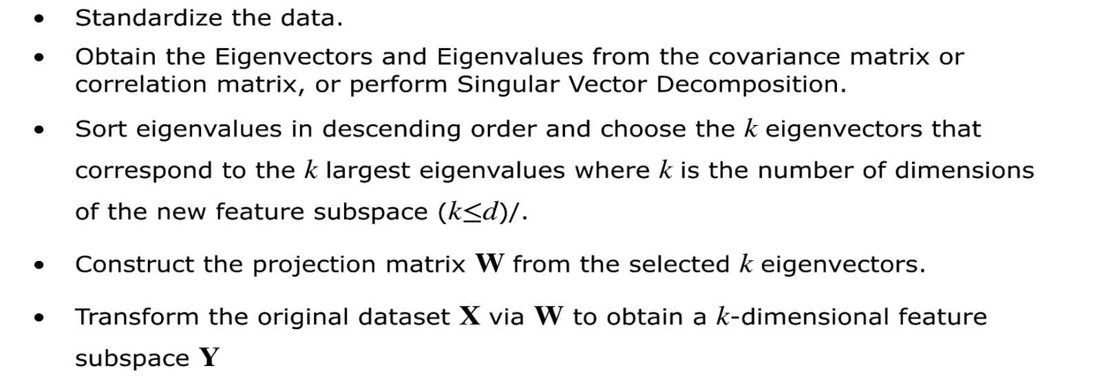
The the main functions of the PCA algorithms are:
Check this page
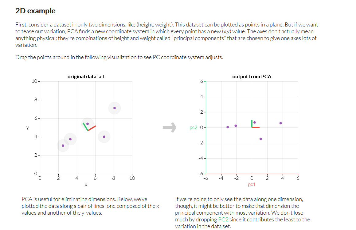
Here you can see 2D image on left and on the right we have 1D image.
You can make changes on left and that will impact on the 1D on right
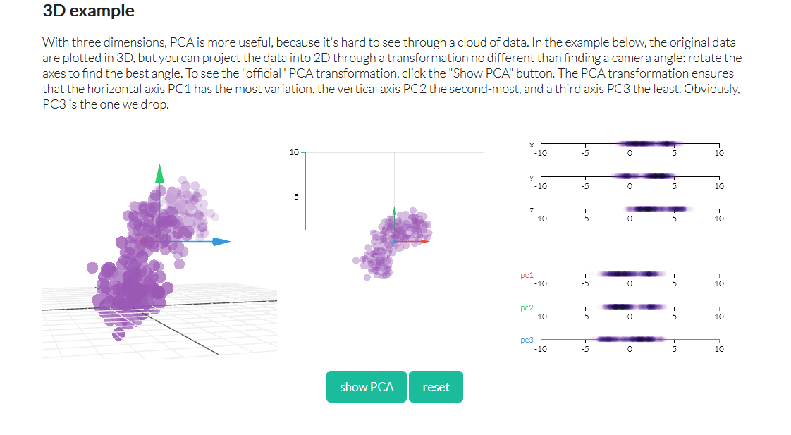
again, here a 3D image has been turned to 2D
Let's code that down
Problem Statement
Here we can see we have various features (column)
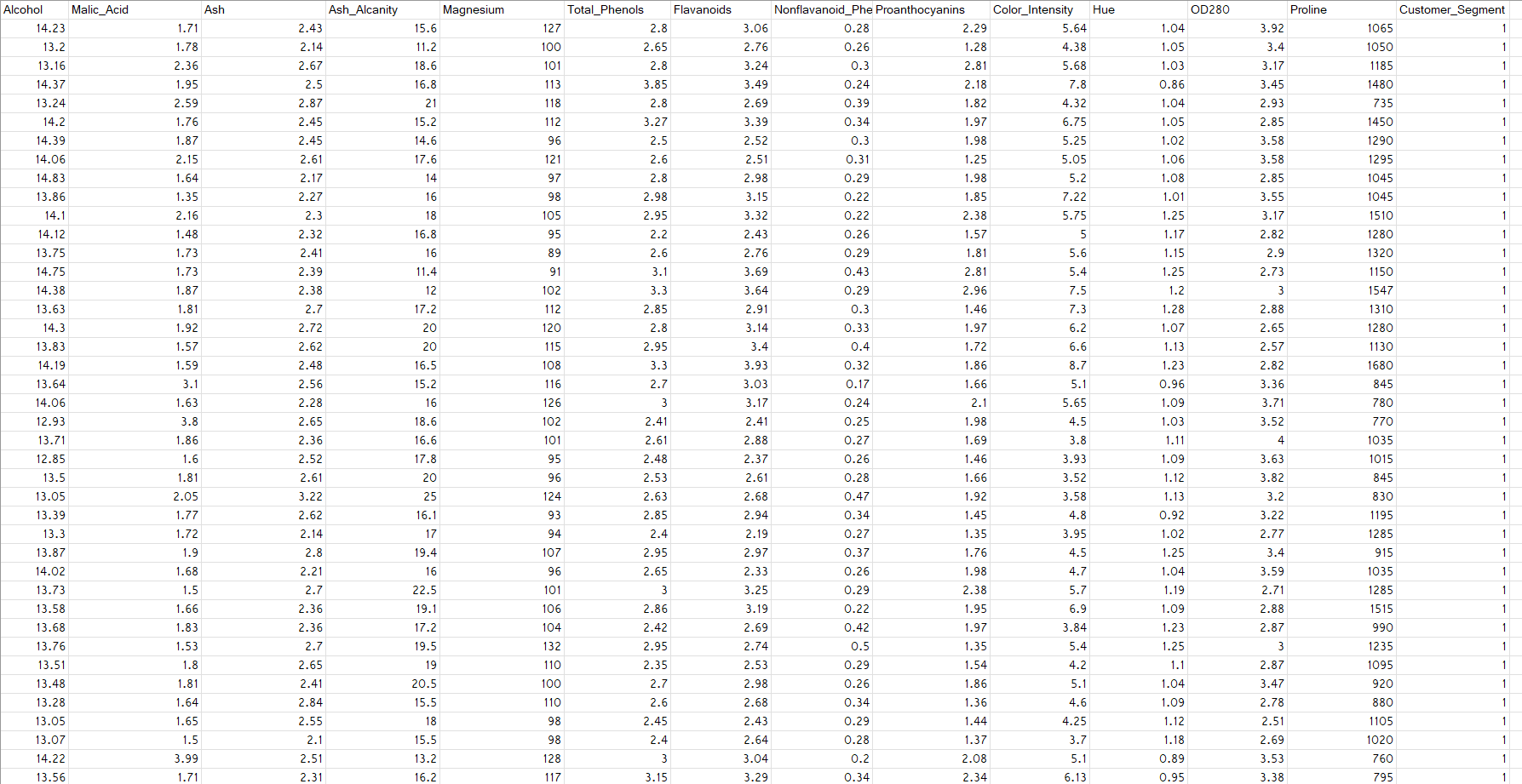
Let's imagine that this data set belongs to a wine merchant with many different bottles of wine to sell and therefore a large base of customers. And this wine shop owner actually hired you as data scientist to first do a preliminary work of clustering.
Here we have 3 customer segment and you can see that in the csv file. And this is the column we will use for y matrix
The owner would like to, reduce the complexity of this data set by ending up with a smaller amount of features. And at the same time, this owner would like you to build a predictive model that will be trained on these data, including the features up to here and the dependent variable,so that for each new wine that this owner has in its shop ,we can deploy this predictive model applied to a reduced dimensionality data set to predict which customer segment this new wine belongs to, right?
And therefore, once we manage to predict which customer segment this wine belongs to then we can recommend this wine to the right customers. And that's exactly why what we're about to do is like a recommender system. Because for each new wine that will be in the shop, well, our predictive model will tell us to which customer segment it will be the most appropriate, it will be the most appreciated.
All right, so that's the business case study. And therefore, our predictive model will add tons of value to this owner.Therefore, if this owner manages to build a good recommender system of course it will optimize the sales and therefore the profit of the business, okay. So that's what the case study is about.
The code is exactly what we have explained previously. So, we will just talk about the PCA part
Let's open the .ipynb file provided below and run the first few cells

Now, if we copy paste this code in spyder IDE, we can see
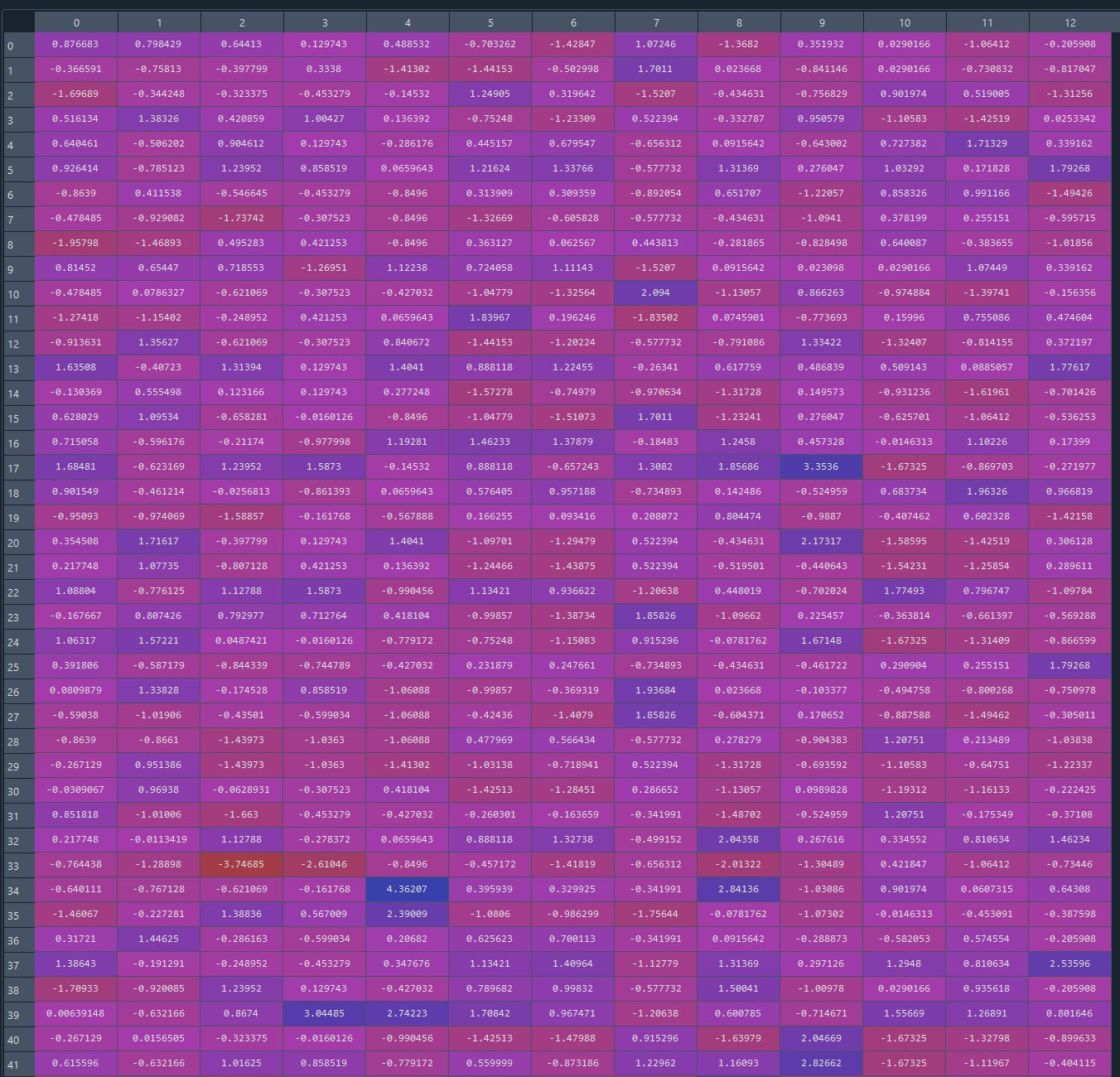
X_train looks like this (with lots of features/column)
X_test looks like this
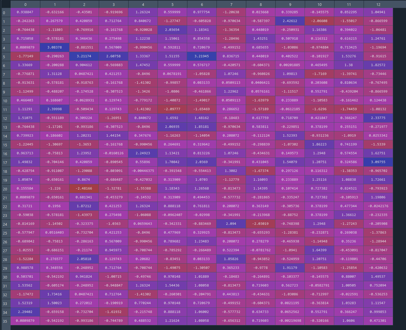
Our goal is to reduce the column/features. Let's start the PCA:
Imported the PCA Class
from sklearn.decomposition import PCA #Importing PCA Class
Now, we will create an object:
pca = PCA() #Created an object
Within the class, we will input our desired dimension/Features. We have lots of features and that will make our plotting much harder and give a huge number of dimension. Our goal is to reduce that and we are going to mention the reduced number of dimension here.So, how many dimension should we have?
Well, I have a very simple answer to that question. What I usually do is start with two. Two principle components, therefore two extracted features and see the results I get in the end.
And thanks to our code, our code template we can check that very quickly and easily. And besides, we do wanna try with two because then if we get good results with two well we will be able to visualize the training set result and test set result in two dimensions, in this nice plot .
pca = PCA(n_components=2)
Then we fit and transform the Xtraining data set
X_train =pca.fit_transform(X_train) #fit and transform the X training set
and (Only transform) then X test set
X_test = pca.transform(X_test)
Using the pca object, we will just transform but not fit because our goal is to check with this data later.
Now, if we run the cell the X_train looks like this
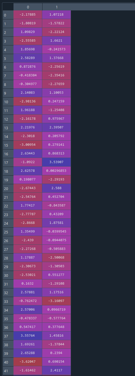
We have only 2 features now due to the PCA. The features has been reduced and dimensions has been reduced as well.
Same goes for X_test
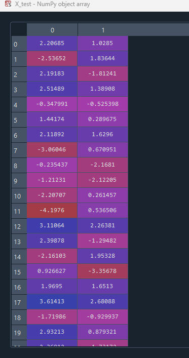
If we fit now, the model will be impacted by the fit
Now, let's run the whole file
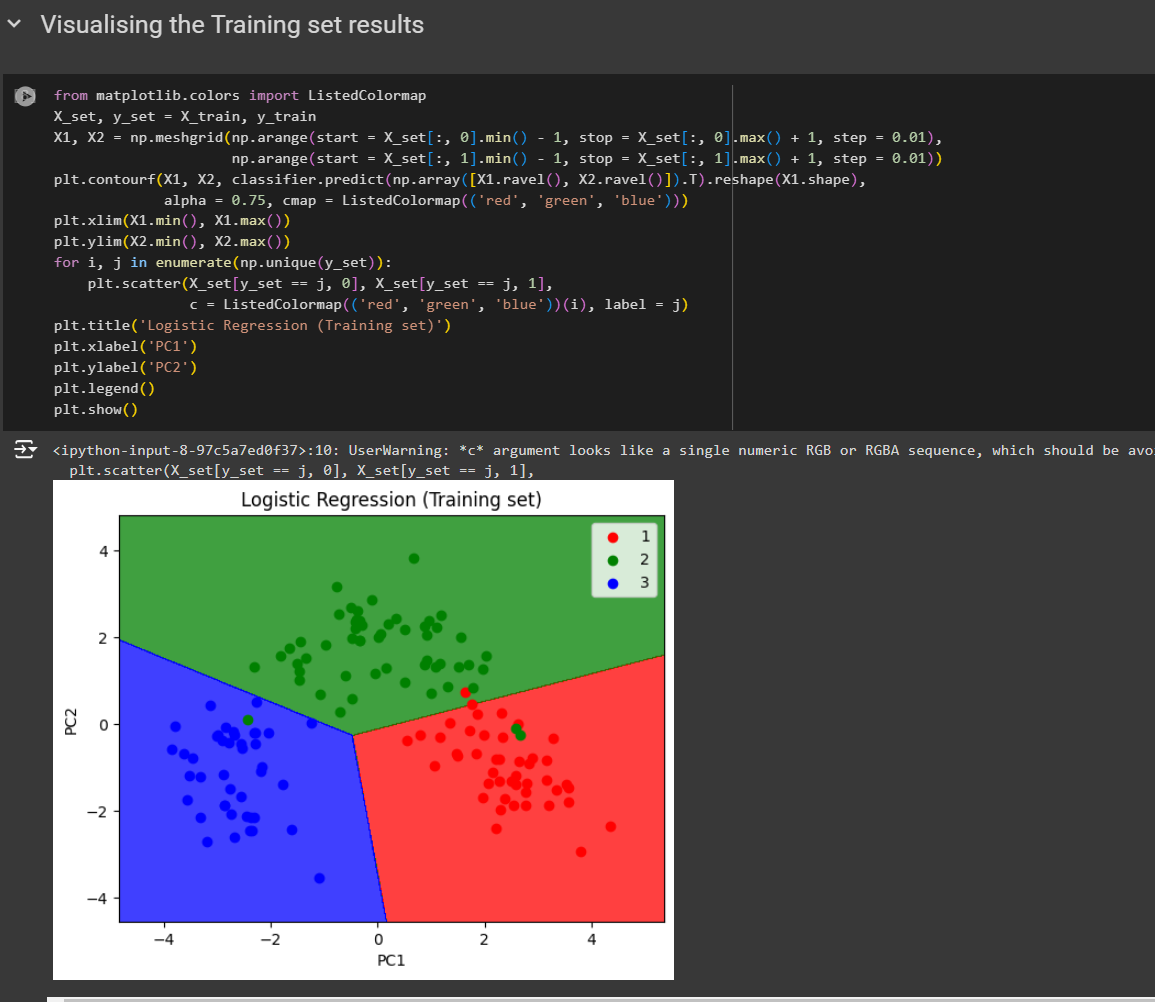
You can see the classification for training set
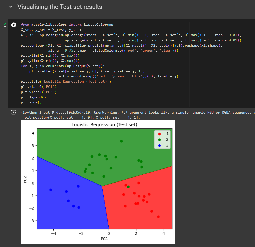
For test set
Note: If you give n_components to any other value than 2, you will find issues as rest of the code was created for 2 feature
You can also apply Kernel PCA (Another form of dimensionality reduction)
from sklearn.decomposition import KernelPCA
kpca = KernelPCA(n_components = 2, kernel = 'rbf')
Here we use radial basis function.
X_train = kpca.fit_transform(X_train)
X_test = kpca.transform(X_test)
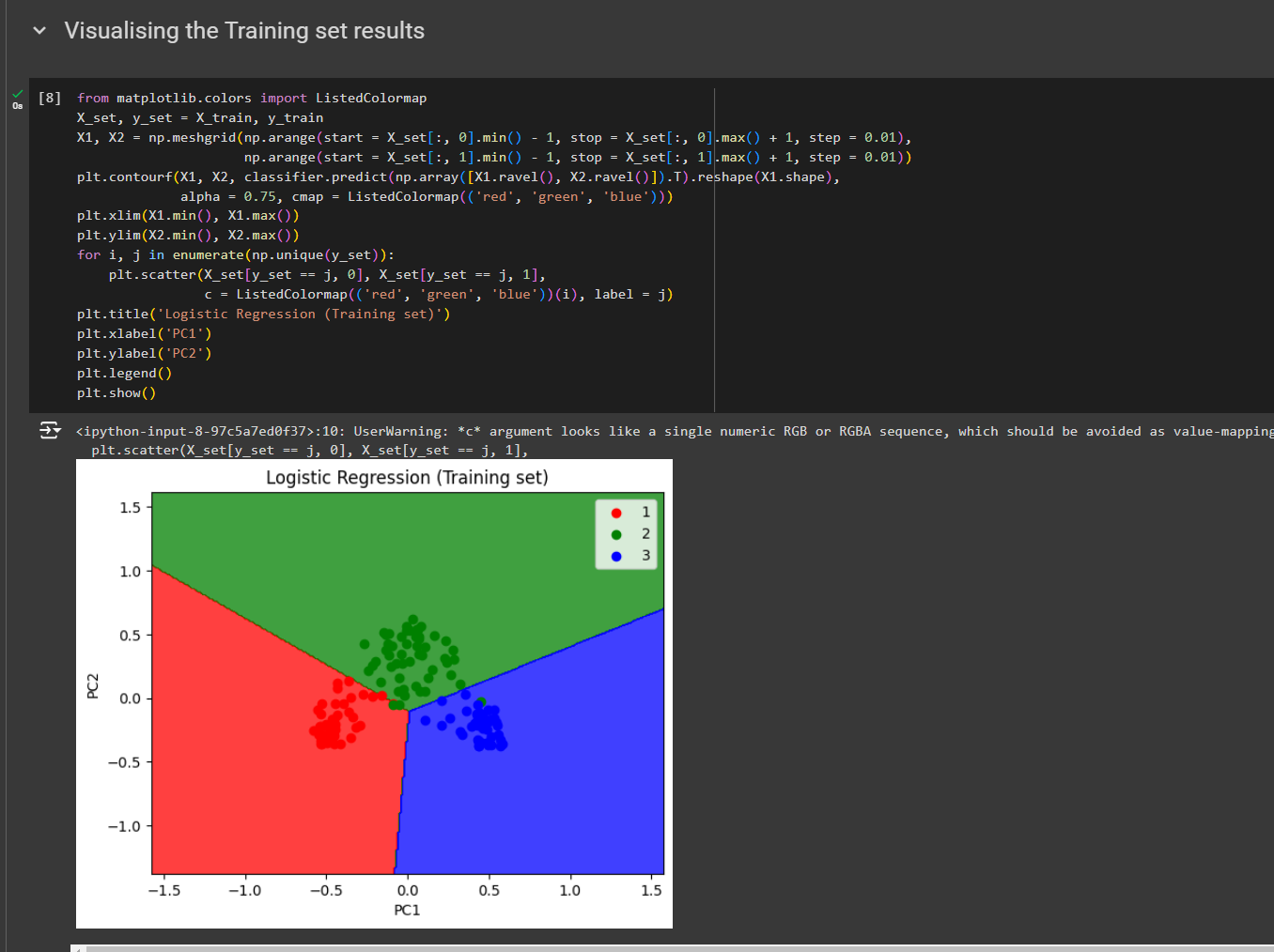
Here the clustering for training data
for test data
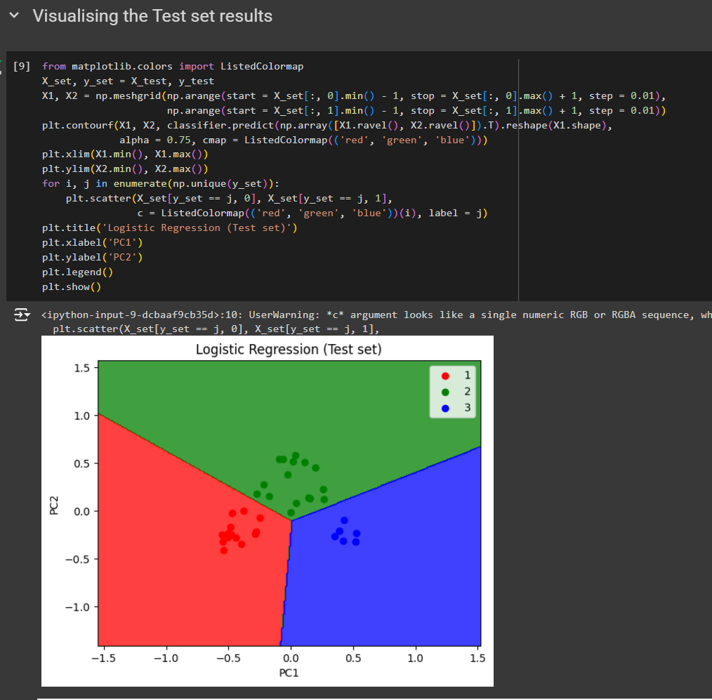
Surely you can see the difference . You can see the points are more close to each other and gives us high chance of prediction.
So, Kernel PCA is better than PCA in this aspect
Code from here
Subscribe to my newsletter
Read articles from Md Shahriyar Al Mustakim Mitul directly inside your inbox. Subscribe to the newsletter, and don't miss out.
Written by
