Machine Learning : Model Selection Techniques, XGBoost (Part 34)

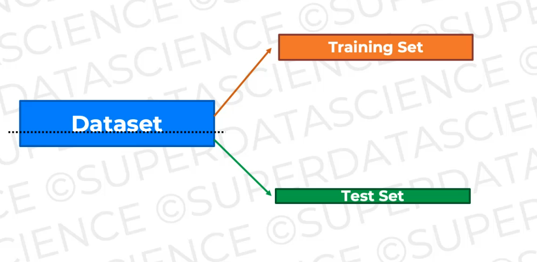
Till now, we have been dividing our main dataset to Training Set and Test set

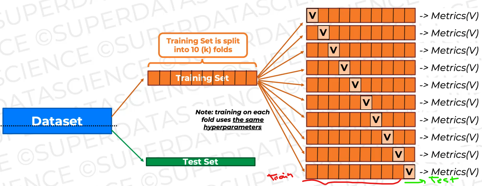
Let's now split the Training set to 10 parts

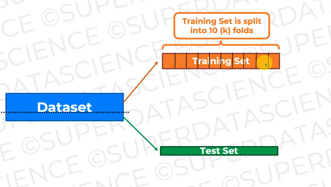
Then what we're going to do is we're going to train the data on nine of these folds and keep one fold as an unseen fold for validation.

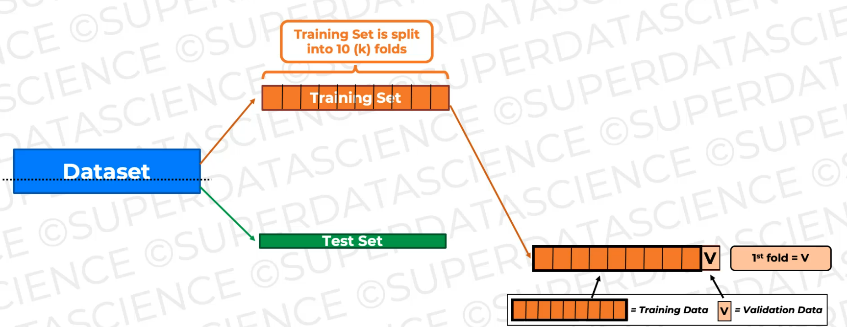
now we're going to shift the validation fold. The validation fold becomes this fold.

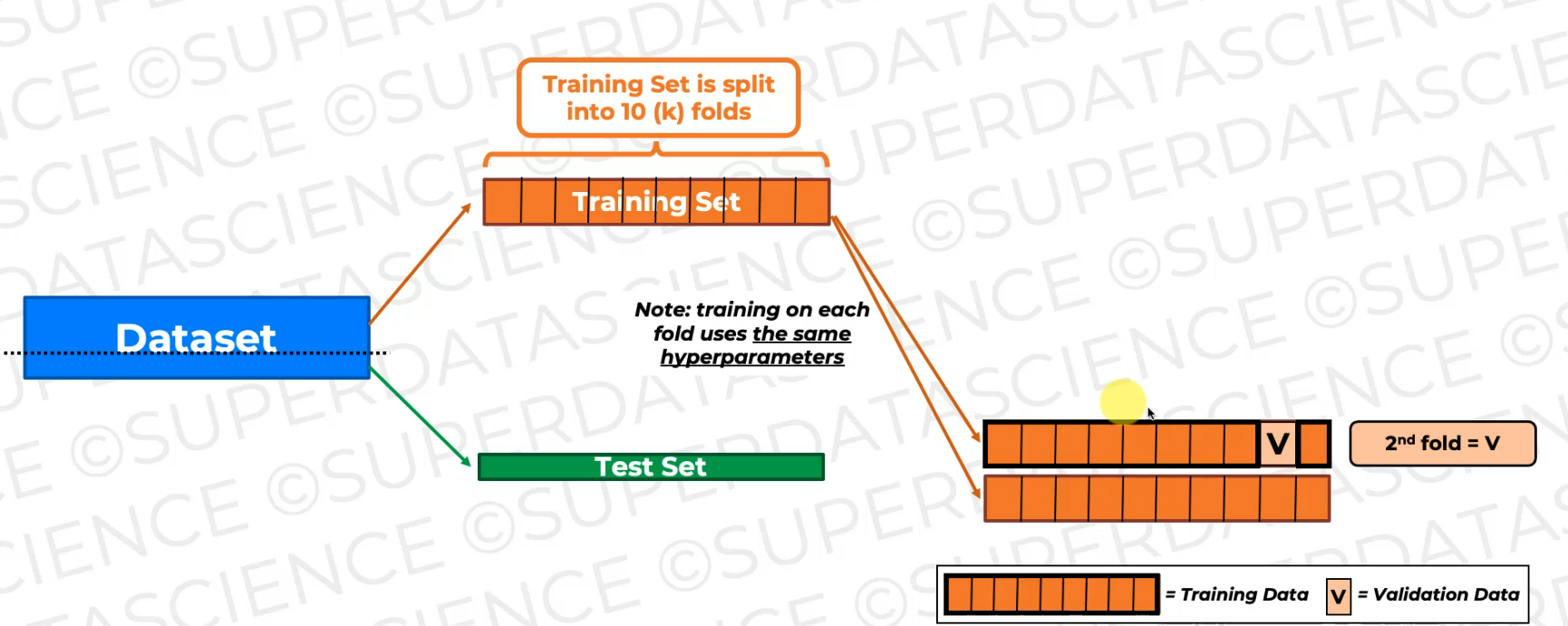
And again, it's not gonna be seen during this training. So we're gonna get a new model as a result of this training, a new trained model, and we're gonna validate on this fold.

And note every time we do this for every fold or every like combination of folds.

So here and here, we have to use the same hyperparameters.

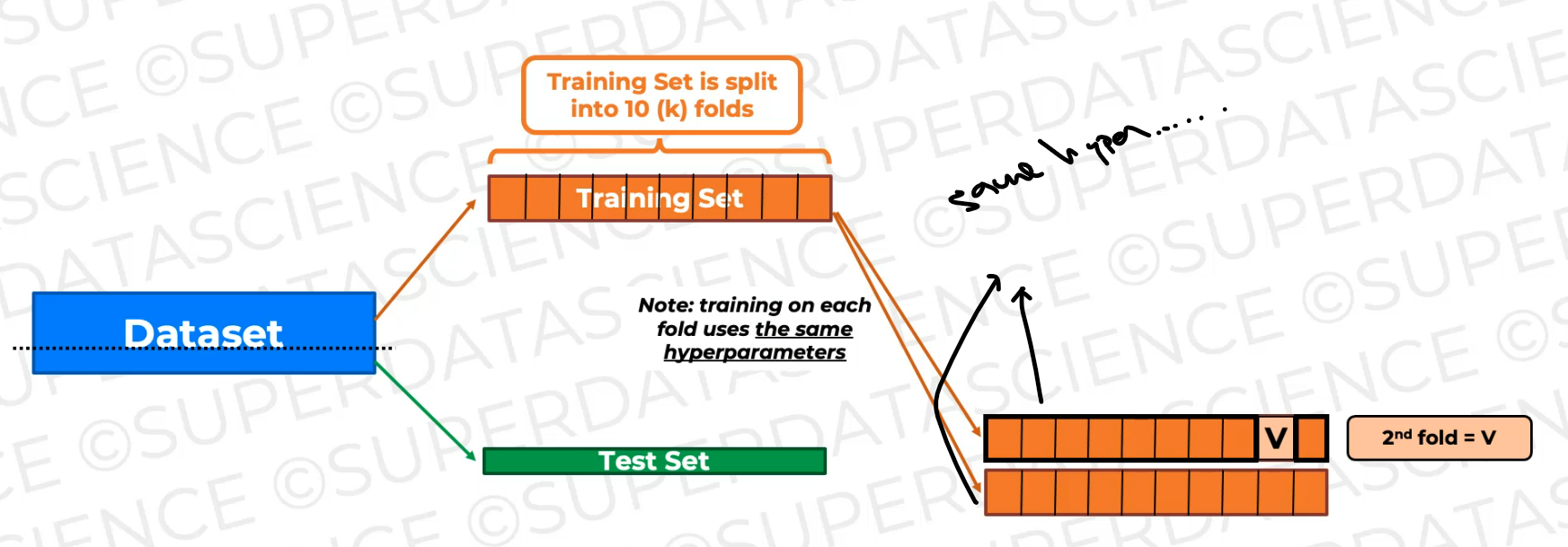
now we're just training the model again and again on slightly different training data and validating it on the validating fold, which is changing, which is shifting as you can see.

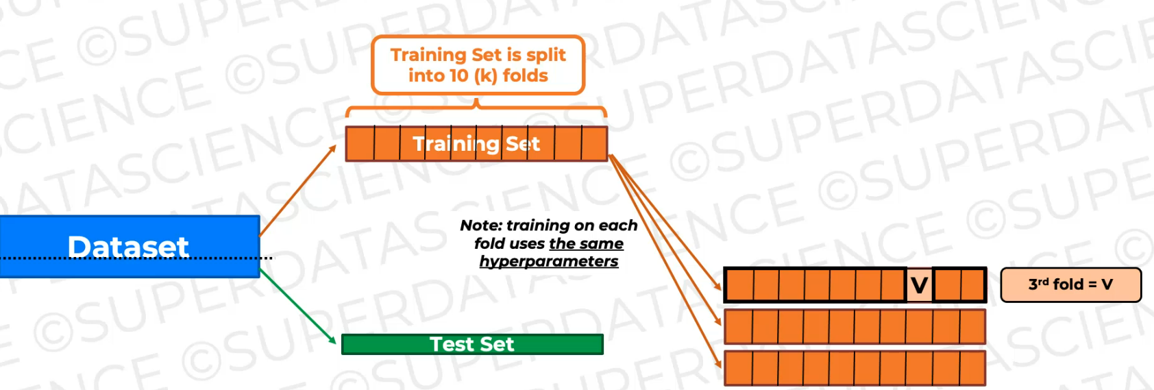
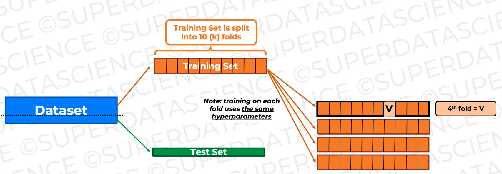
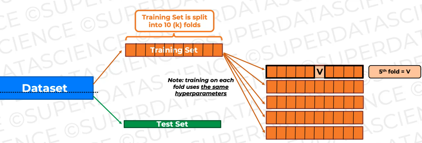
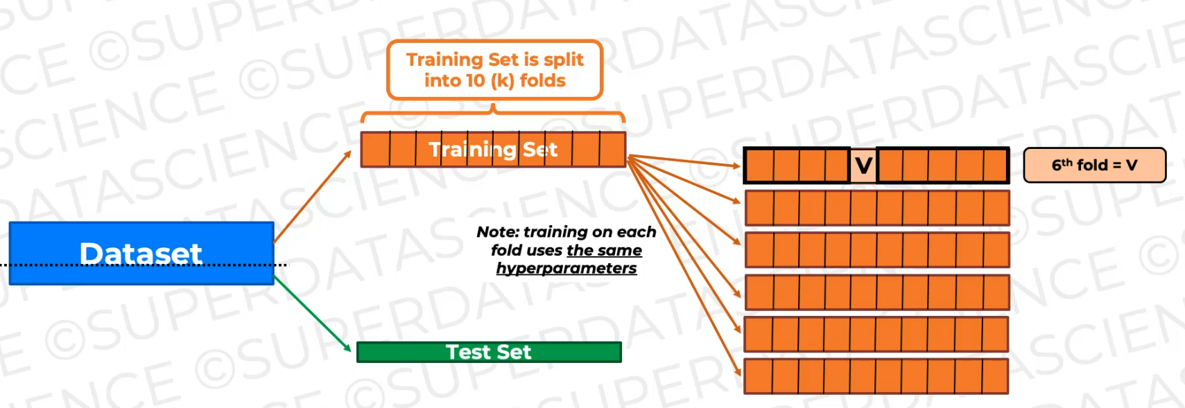
So here's our six training.

So we train it on all of this data and then validate it on this fold (every time it's different), which is not seen during training.

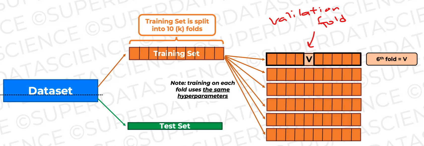
And as a result, we will have 10 sets of metrics.

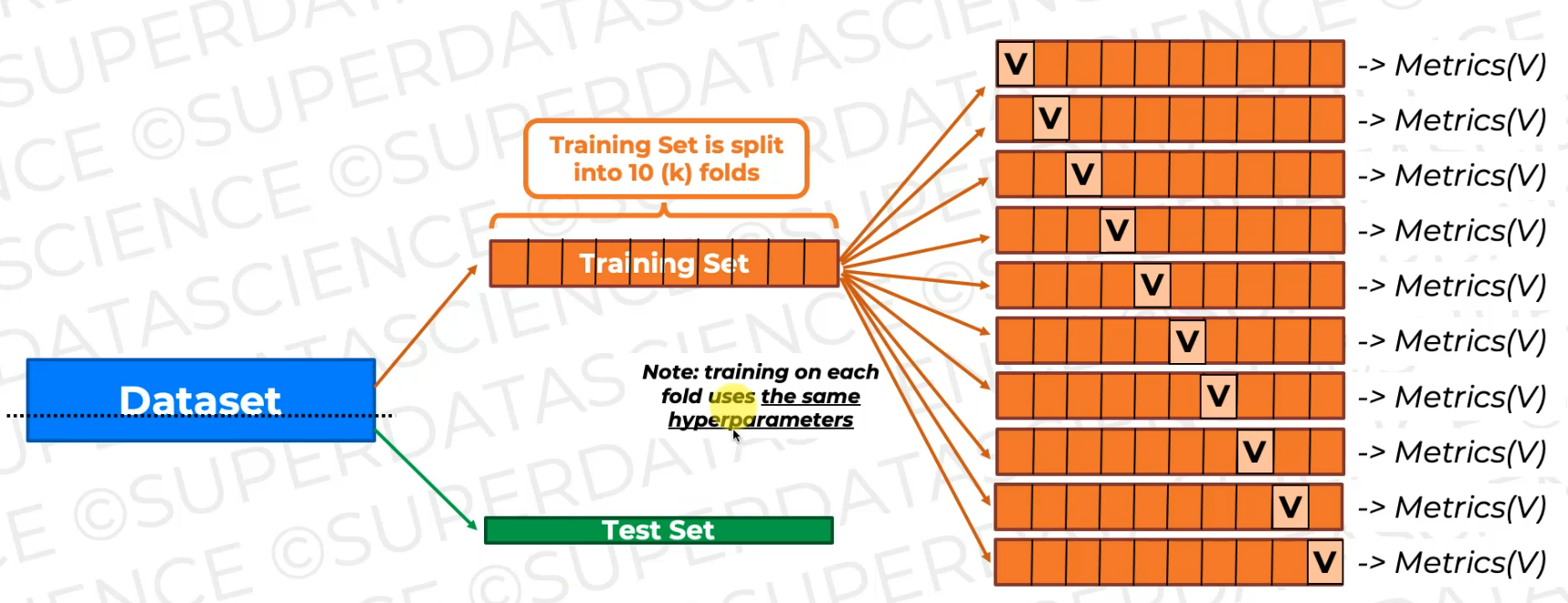
we're going to have 10 sets of metrics and we can look at them and aggregate

So let's make some space and here we're going to assess these metrics and look at them in aggregate. And if these metrics look good in aggregate, then the modeling approach is valid. So the model you've selected and the hyperparameters you selected are good for this data.

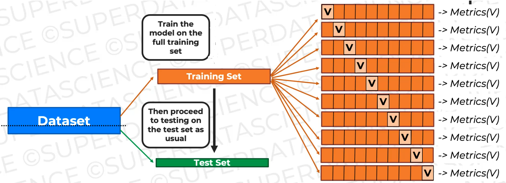
And then what we're going to do is we're going to train the model. This time we're gonna train on all of the training data and then **we're going to test it on the test set as usual.**That's our final step.

On the other hand, if the aggregate metrics don't look good, then something's wrong, then otherwise, we need to, adjust hyperparameters of the model or we have to change the model entirely

Code:

Bias Variance Tradeoff

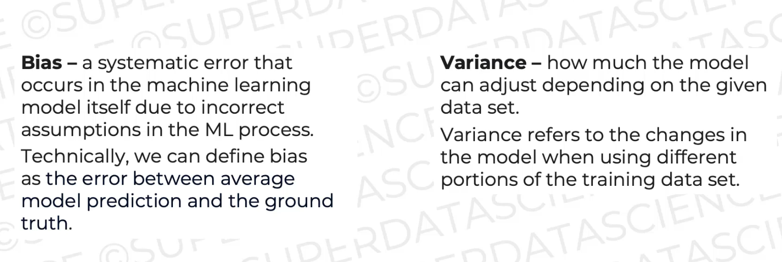
Let's understand what is Bias and what is Variance

Let's see what have we learned so far
We split our set, we've got our training set, then the training set was split into 10 folds. And so then, we train the model on these nine folds combined and we validate it or do tests on this one leftover fold. Then, we train the model on these nine folds, and then we test it on this one fold.

if we plot this on the bias-variance curve,this is what happens when you have high bias, low variance.

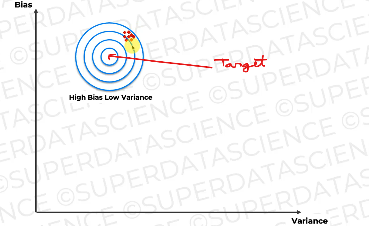
This is what you want to predict, this is the target, but your model is all of those predictions of all those models that we just looked at. They are far away from the target, but they're clustered together, right?

And what does that mean?

Well, that means that the model is too simple and does not capture the underlying trend of the data.

On the other hand, you might have this situation where you have low bias and high variance where the average of all of these models is on the target

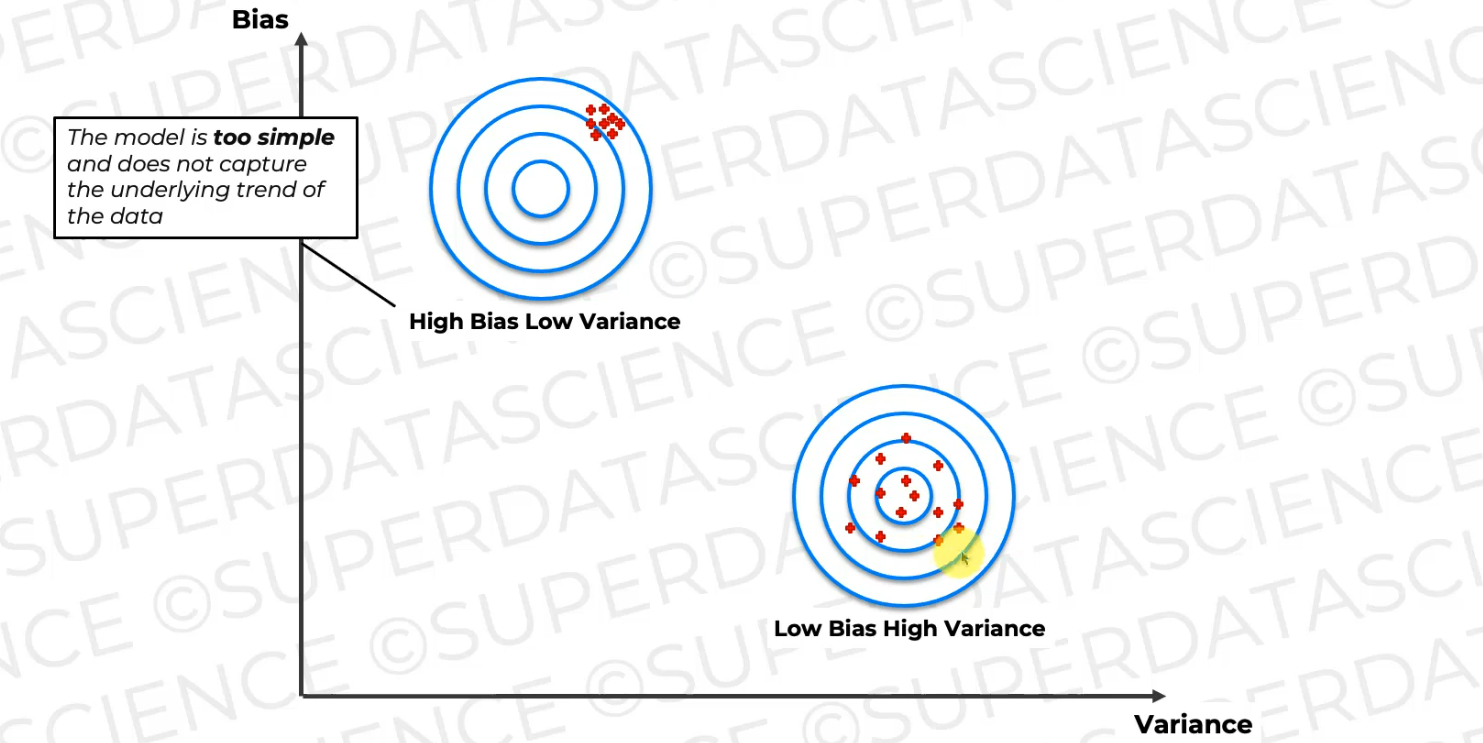
every time we change the underlying trained data slightly, the model result is different or it varies.

And both of these scenarios, as you can imagine, are bad.

You can also have a scenario like this where you have high bias and high variance, so the average of these predictions is somewhere here, which is also away from where we want it to be, and they're also scattered across.

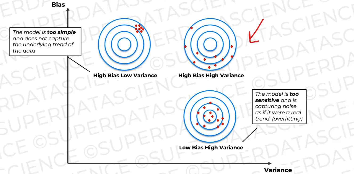
And this is the probably the worst of the three, and here, the model is too simple to capture the data's trend and it's too sensitive, it captures noise as well.

Here's the ideal scenario,

which is kind of like the unicorn

where your data is clustered together,

so you have low variance and it's in the right spot around.

So the average is the average that we want,

actually, we're aiming to predict,

so therefore it's got low bias.

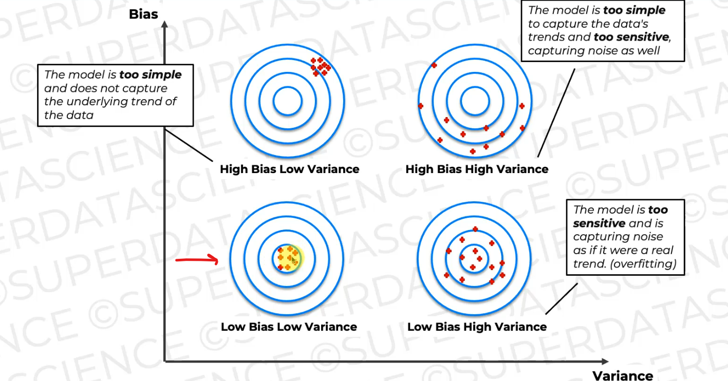
And this is a great model, it accurately captures the underlying trends of the data and generalizes well to unseen data.

Now, the thing is that this is very rare and it's kind of like a unicorn to catch this kind of scenario.

We mostly get High bias low variance or Low Bias High Variance and make changes and changes to get Low Bias Low Variance.

Let's code this down with a CSV file

from sklearn.model_selection import cross_val_score # cross_val_score is a function accuracies = cross_val_score(estimator = classifier, X = X_train, y = y_train, cv = 10) Here, 10 is the number of folds

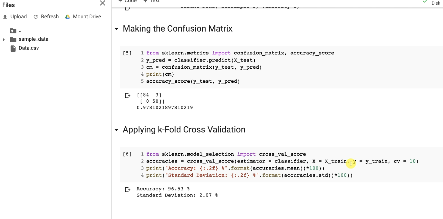
print("Accuracy: {:.2f} %".format(accuracies.mean()*100)) #mean of the accuracies print("Standard Deviation: {:.2f} %".format(accuracies.std()*100)) #standard deviation of the accuracies

Once we run this, we get

Just running this will give us the mean of the 10 accuracies of this accuracies vector. So, we get 90%. That means that the mean of these 10 accuracies here is actually 90%. And so in conclusion, this 90% accuracy is the relevant evaluation of our model performance.

And we get a 6% standard deviation. So what does that mean?

That means that the average of the differences between the different accuracies that we'll get when evaluating our model performance and the average accuracy, that is 90%, is 6%.

So that's actually not too high variance. That's okay, because that means that when we evaluate our model performance, well, most of the time we will be around 84% and 96%

So eventually, that means that we are in this low bias and low variance category

Code here

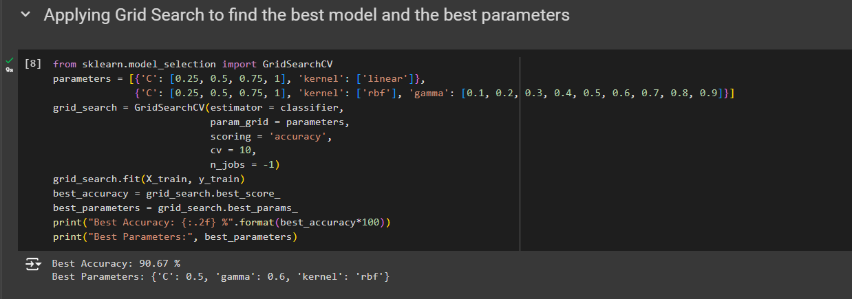
There is another method - Grid Search

from sklearn.model_selection import GridSearchCV

parameters = [{'C': [0.25, 0.5, 0.75, 1], 'kernel': ['linear']},

{'C': [0.25, 0.5, 0.75, 1], 'kernel': ['rbf'], 'gamma': [0.1, 0.2, 0.3, 0.4, 0.5, 0.6, 0.7, 0.8, 0.9]}]

grid_search = GridSearchCV(estimator = classifier,

param_grid = parameters,

scoring = 'accuracy',

cv = 10,

n_jobs = -1)

grid_search.fit(X_train, y_train)

best_accuracy = grid_search.best_score_

best_parameters = grid_search.best_params_

print("Best Accuracy: {:.2f} %".format(best_accuracy*100))

print("Best Parameters:", best_parameters)

After running that, we got this

We have taken 2 sets of values,

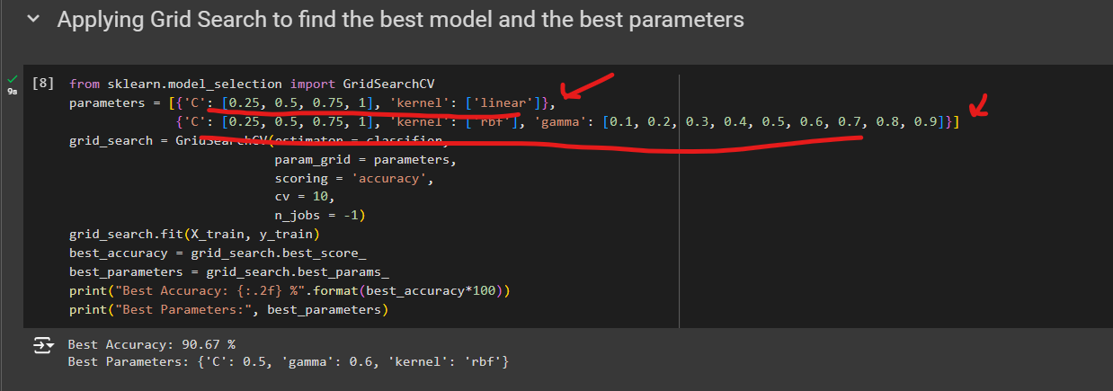
We will check for which of the values (These values have been taken based on our experience and you will learn about them as you learn more), we get a better accuracy.

We get a best accuracy of 90.67%, which is slightly better than this, 90.33%.

But you will see in your future machinery projects that even a slight improvement of the accuracy can make a difference. And the best combination of parameters that led to that best accuracy is the following first regularization parameters C of 0.5, meaning that indeed it was necessary to reduce a bit that hyper parameters C to reduce overfitting.

Then of course we got the best accuracy with an RBF kernel And the best value of this gamma parameter, you know when we have a RBF kernel is indeed 0.6.

Code from here

XGBoost

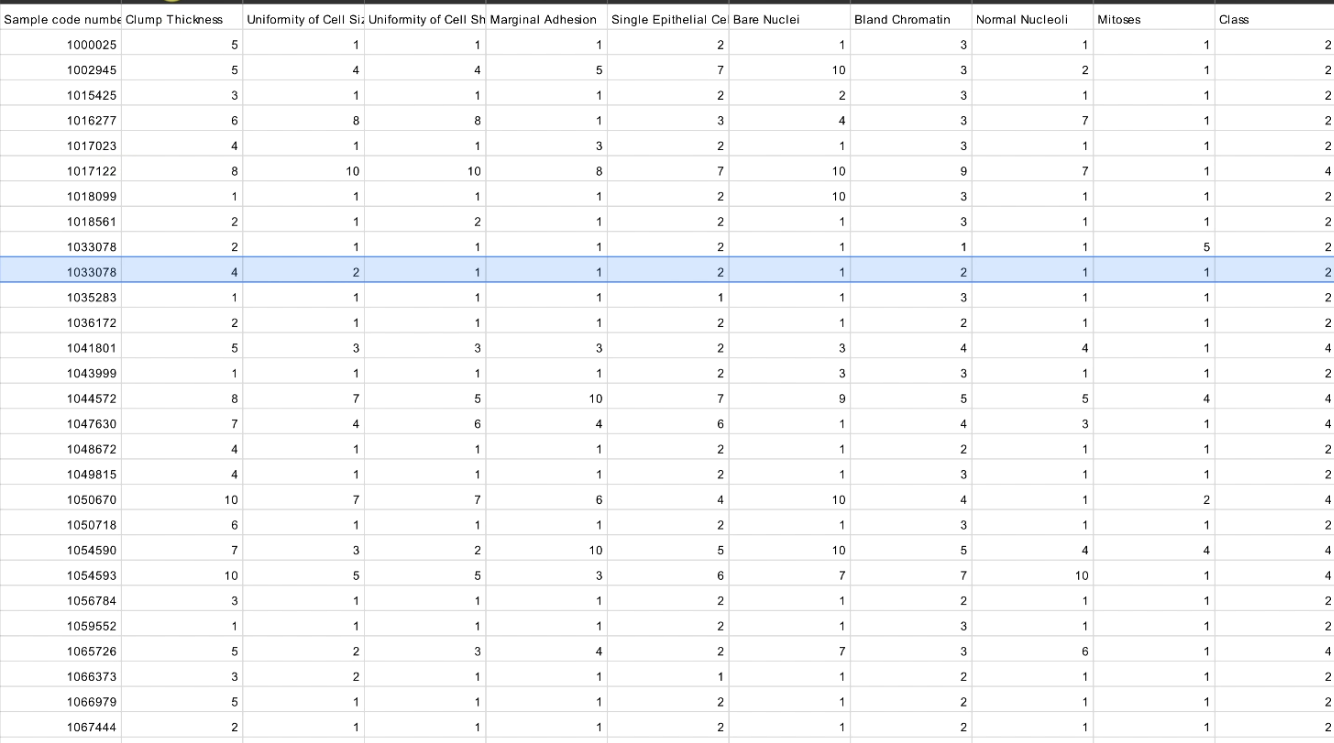
Here from the dataset, we will detect if a breast cancer tumor is benign or malignant,

meaning that each row of this dataset corresponds to a patient, and for each of these patients, we have several features, from the clump thickness, the uniformity of cell size, the uniformity of cell shape, you know, all these features that are characteristics of a tumor.

We were trying to predict if the tumor is benign or malignant. It is benign if we get the class two (2), and malignant if we get the class four (4)

With the logistic regression model, we had an accuracy of 94.7%. with the k-Nearest Neighbors, we had an accuracy of 94.7% again. With the SVM we had an accuracy of 94.1%. With the kernel SVM, we had a better accuracy actually with 95.3%. With Naive Bayes we got a lower accuracy of 94.1% again, and with decision tree classification well, that was the winner. We got an amazing accuracy of 95.9%. That was the number one on the podium, followed by the kernel SVM with that accuracy. And then, unfortunately, random forests did not do any good, or you know, not better than the others, because we got a 93.5% accuracy with it. [Note: In my earlier blogs, I have applied these models using the same dataset and got these results]

And so, what I wanna do now, as you probably have guessed, is to build the XGBoost model and train it on the same dataset to see if it can take the throne hold by the decision tree classification model. In other words, to see if it can beat that accuracy obtained with the decision tree classification model.

from xgboost import XGBClassifier

classifier = XGBClassifier()

classifier.fit(X_train, y_train)

and we get an impressive accuracy of 97.8% (In the confusion matrix)

So, it's far better than the decision tree

Code here