Predicting House Prices: How Size Influences Market Value

In this project, say I worked for a client who wanted to create a model to predict apartment prices in Buenos Aires, focusing on properties under $500,000 USD. To streamline the data importing and cleaning process, I wrote a custom function to ensure consistency across all datasets. This approach not only standardizes the analysis but also enhances reproducibility—crucial in both science and data science. The necessary libraries were imported, and a function named "load" was created, which takes a file path as input and returns a cleaned DataFrame ready for analysis.

def load(file_path):
    # Load the data
    df = pd.read_csv(file_path)

    # Return the dataframe
    return df

# The file path
file_path = (r"C:\Users\user222\OneDrive\Documents\Data Analysis\WQU\Datasets\Buenos Aires\buenos-aires-real-estate-1.csv")

For this project, the focus was to build a model for apartments in Buenos Aires proper ("Capital Federal") that cost less than $500,000. Below is the first few rows of the imported dataset. It consists of 8606 rows and 16 columns.

For the initial data cleaning task, there was need to remove any observations exceeding $500,000 from the dataset. Since the project was utilizing a function to import and clean the data, there was need to update this function accordingly. Additionally, I’ve adjusted the load function to ensure that the DataFrame it returns only includes records related to "apartments" in Buenos Aires ("Capital Federal"). To make this process more transparent, I've highlighted the relevant columns for easier viewing.

def load(file_path):
    # Load the data
    df = pd.read_csv(file_path)
    # Subset data: Apartments in "Capital Federal", less than 400,000
    mask_ba = df["place_with_parent_names"].str.contains("Capital Federal")
    # Include only apartment property type
    mask_apt = df["property_type"] == "apartment"
    # Include only prices less than $500,00
    mask_price = df["price_aprox_usd"] < 500_000
    # Ensures that these changes are done to the dataframe
    df = df[mask_ba & mask_apt & mask_price]

    # Return the dataframe
    return df
# The file path
file_path = (r"C:\Users\user222\OneDrive\Documents\Data Analysis\WQU\Datasets\Buenos Aires\buenos-aires-real-estate-1.csv")

The resulting dataframe is shown below with 1829 rows and 16 columns.

A histogram of "surface_covered_in_m2" was created to have quick distribution to prepare for more data cleaning. The x-axis has the label "Area [sq meters]" and the plot has the title "Distribution of Apartment Sizes". Below is the histogram

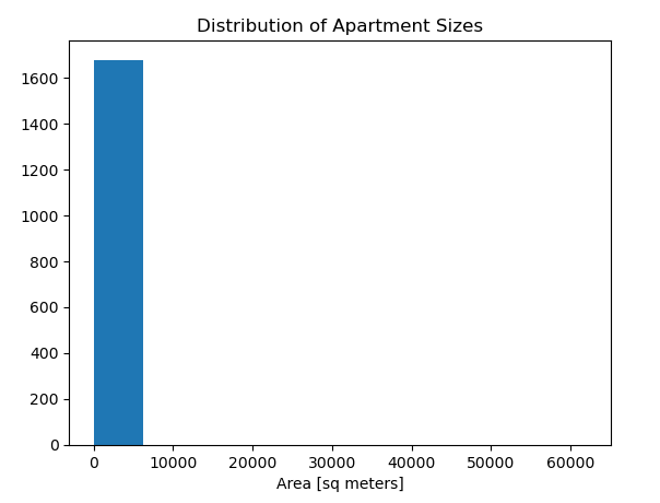
Histograms, such as the one shown above, indicates the presence of outliers in the dataset. These outliers can significantly impact the performance of linear models, which are central to the analysis in this project. To verify this, let’s examine the summary statistics for the "surface_covered_in_m2" feature. The result is shown below

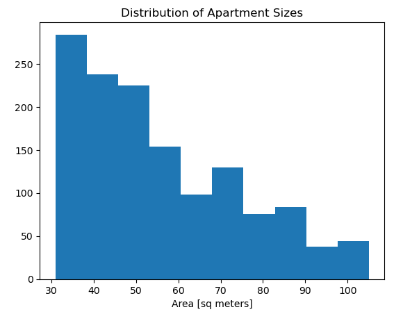
Observing the difference between the mean (approximately 98 square meters) and the maximum (62,034 square meters), along with the 75th percentile at 75 square meters, suggests that while most apartments are relatively small, the large maximum value points to the presence of outliers. To address this, a code was added to the function to filter out outliers, retaining only the data within the 0.1 to 0.9 percentile range. The importing process has been updated accordingly. The histogram was plotted again.

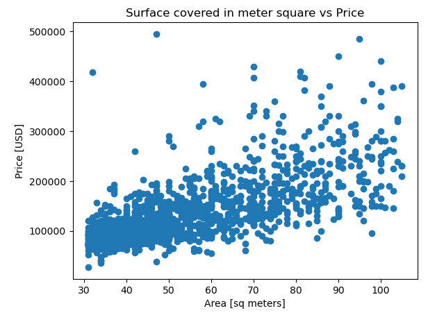
Exploration on the relationship between apartment size and price was done with the use of a scatter plot. The scatter plot shows price ("price_aprox_usd") vs area ("surface_covered_in_m2") in the dataset. The x-axis was labeled "Area [sq meters]", y-axis "Price [USD]", and title "Surface covered in meter square vs Price".

SPLIT

A crucial step in any model-building project is distinguishing between your target variable (the outcome you want to predict) and your features (the information your model uses to make predictions). In this project, which aims to predict price based on apartment size, apartment size serves as the feature. A feature matrix called X_train, was used for training the model, which includes only one feature: ["surface_covered_in_m2"]. Additionally, a target vector named y_train was established, which contains the values for "price_aprox_usd" and was used to train the model.

# Feature matrix
features =  ["surface_covered_in_m2"]
X_train =  df[features]
# Target vector
target = "price_aprox_usd"
y_train = df[target]

MODEL BUILDING (Baseline Model)

The initial step in building a model is establishing a baseline to gauge its performance. This involves evaluating how a simple or "dumb" model would fare on the same data. Often referred to as a naïve or baseline model, this approach makes a single prediction for all instances—predicting the same price irrespective of the apartment size. To create this baseline, the mean of the target vector y_train was calculated. The resulting baseline prediction was 139,268.31. The code used to determine this baseline prediction is provided below.

# Baseline prediction of y_train
y_mean = y_train.mean()
y_mean

After the baseline prediction that the dumb model will always make, it is needed to generate a list that repeats the prediction for every observation in our dataset. To achieve this, a list named y_pred_baseline was created, it contains the value of y_mean repeated so that it's the same length at y.

# A list that generates a prediction for each observation in the dataset 
y_pred_baseline = [y_mean] * len(y_train)

To check how the baseline model performs, one way to evaluate it is by plotting it on top of the scatter plot made above. A line was added to the plot below that shows the relationship between the observations X_train and the dumb model's predictions y_pred_baseline. The line color is orange, and it also has the label "Baseline Model".

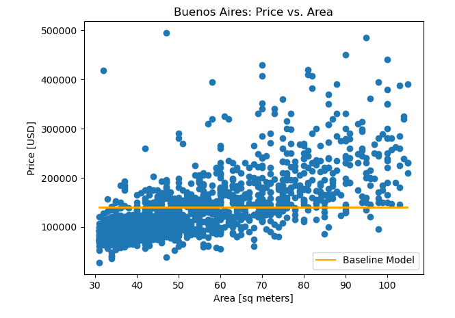
Looking at this visualization, the baseline model doesn't really follow the trend in the data. There are lots of performance metrics that can be used to evaluate a model, but this project uses the mean absolute error. The baseline mean absolute error for the predictions were calculated in y_pred_baseline as compared to the true targets in y.

This information tells us that if we always predicted that an apartment price is $139,268.31, our predictions would be off by an average of $48,756.9. It also tells us that our model needs to have mean absolute error below $48,756.9 in order to be useful.

The next step in building the model is iterating. This involves building a model, training it, evaluating it, and then repeating the process until one is happy with the model's performance. Even though the model in this project is linear, the iteration process rarely follows a straight line. Sometimes, trying new things, hitting dead-ends, and waiting around while your computer does long computations to train your model is inevitable.

The model was created by Instantiating a LinearRegression model named model. The imported data was then used to train the model (fitting the model to the training data).

EVALUATE

The model was then evaluated by making predictions for data that it saw during training. The prices for the houses in our training set was predicted using the model's predict method, a list of predictions for the observations in the feature matrix X_train was created and named y_pred_training.

The predictions were then used to assess our model's performance with the training data. Same metric used to evaluate the baseline model: mean absolute error was used to calculate the training mean absolute error for the predictions in y_pred_training as compared to the true targets in y_train.

The value was 33402.03. beating the baseline by over $15,000.

A test data was introduced into the model to generate a series of predictions using the code below.

# Importing a test data so the model can make predictions

X_test = pd.read_csv(r"C:\Users\user222\OneDrive\Documents\Data Analysis\WQU\Datasets\Buenos Aires\ba-test-data.csv")[features]
y_pred_test = pd.Series(model.predict(X_test))
y_pred_test.head()

The intercept and coefficient were gotten to show equation that the model has determined for predicting apartment price based on size. For visualization, the line that shows the relationship between the observations in X_train and the model's predictions y_pred_training was plotted on the scatter plot created at the beginning of this project.

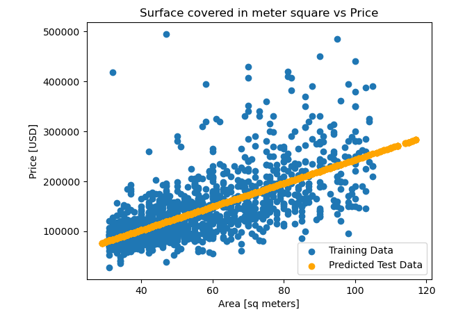
The linear regression model was able to predict apartment prices based on size with reasonable accuracy, outperforming the baseline model. However, further refinement and inclusion of additional features could potentially improve the model's performance.

For the detailed codes used for this analysis, visit my Github repository here.

For collaborations and questions, reach out to me via my LinkedIn page here.