Comparing Brazilian and US university theses using natural language processing
 freeCodeCamp
By Déborah Mesquita
People are more likely to consider a thesis that’s written by a student at a top-ranked University as better than a thesis produced by a student at a University with low (or no) status.
But in what way are the works different? What can the students from non-famous Universities do to produce better work and become more well-known?
I was curious to answer these questions, so I decided to explore two things only: the themes of the works and their nature. Measuring the quality of a university is something very complex, and is not my goal here. We will analyze a number of Undergraduate theses using natural language processing. We’ll extract keywords using tf-idf and classify the theses using Latent Semantic Indexing (LSI).
The data
Our dataset has abstracts of Undergraduate Computer Science Theses from Federal University of Pernambuco (UFPE), located in Brazil, and from Carnegie Mellon University, located in the United States. Why Carnegie Mellon? Because it was the only University where I could find a list of theses produced by students who were at the end of their Undergraduate degree program.
The Times Higher Education World University Rankings says that Carnegie Mellon has the 6th best Computer Science program, while UFPE is not event in this ranking. Carnegie Mellon ranks 23rd in the World University Ranking, and UFPE is around 801st.
All works were produced between the years of 2002 and 2016. Each thesis has the following information:
- title of the thesis
- abstract of the thesis
- year of the thesis
- university where the thesis was produced
Theses from Carnegie Mellon can be found here and theses from Federal University of Pernambuco can be found here.
Step 1 — Investigating the themes of the theses
Extracting keywords
To get the themes of the thesis, we will use a well known algorithm called tf-idf.
tf-idf
What tf-idf does is to penalize words that appear a lot in a document and at the same time appear a lot in other documents. If this happens, the word is not a good pick to characterize this text (as the word could also be used to characterize all the texts). Let’s use an example to understand this better. We have two documents:
Document 1:
| Term | Term Count | |--------|------------| | this | 1 | | is | 1 | | a | 2 | | sample | 1 |
And Document 2:
| Term | Term Count | |---------|------------| | this | 1 | | is | 1 | | another | 2 | | example | 3 |
First let’s see what’s going on. The word this appears 1 time in both documents. This could mean that the word is kind of neutral, right?
On the other hand, the word example appears 3 times in Document 2 and 0 times in Document 1. Interesting.
Now let’s apply some math. We need to compute two things: TF (Term Frequency) and IDF (Inverse Document Frequency).
The equation for TF is:
TF(t) = (Number of times that term t appears in the document) / (Total number of terms in the document)
So for terms this and example, we have:
TF('this', Document 1) = 1/5 = 0.2TF('example',Document 1) = 0/5 = 0
TF('this', Document 2) = 1/7 = 0.14TF('example',Document 2) = 3/7 = 0.43
The equation for IDF is:
IDF(t) = log_e(Total number of documents / Number of documents where term t is present)
Why do we use a logarithm here? Because tf-idf is is an heuristic.
The intuition was that a query term which occurs in many documents is not a good discriminator, and should be given less weight than one which occurs in few documents, and the measure was an heuristic implementation of this intuition. — Stephen Robertson
The aspect emphasised is that the relevance of a term or a document does not increase proportionally with term (or document) frequency. Using a sub-linear function (the logarithm) therefore helps dumped down (sic) this effect. …The influence of very large or very small values (e.g. very rare words) is also amortised. — usεr11852
Using the equation for IDF, we have:
IDF('this', Documents) = log(2/2) = 0
IDF('example',Documents) = log(2/1) = 0.30
And finally, the TF-IDF:
TF-IDF('this', Document 2) = 0.14 x 0 = 0TF-IDF('example',Document 2) = 0.43 x 0.30 = 0.13
I used the 4 words with highest scores results from the tf-idf algorithm for each thesis. I did this using CountVectorizer and TfidfTransformer from scikit-learn.
You can see the Jupyter notebook with the code here.
With 4 keywords for each thesis, I used the WordCloud library to visualize the words for each University.


Topic Modeling
Another strategy I used to explore the themes from theses of both Universities was topic modeling with Latent Semantic Indexing (LSI).
Latent Semantic Indexing
This algorithm gets data from tf-idf and uses matrix decomposition to group documents in topics. We will need some linear algebra to understand this, so let’s start.
Singular Value Decomposition (SVD)
First we need to define how to do this matrix decomposition. We will use Singular Value Decomposition (SVD). Given a matrix M of dimensions m x n, M can be described as:
M = UDV*
Where U and V* are orthonormal basis (V* represents the transpose of matrix V). An orthonormal basis is the result if we have two things (normal + orthogonal):
- when all vectors are of length 1
- when all vectors are mutually orthogonal (they make an angle of 90°)
D is a diagonal matrix (the entries outside the main diagonal are all zero).
To get a sense of how all of this works together we will use the brilliant geometric explanation from this article by David Austing.
Let’s say we have a matrix M:
M = | 3 0 | | 0 1 |
We can take a point (x,y) in the plane and transforming it into another point using matrix multiplication:
| 3 0 | . | x | = | 3x || 0 1 | | y | | y |
The effect of this transformation is shown below:


As we can see, the plane is horizontally stretched by a factor of 3, while there is no vertical change.
Now, if we take another matrix, M’:
M' = | 2 1 | | 1 2 |
The effect is:


It is not so clear how to simply describe the geometric effect of the transformation. However, let’s rotate our grid through a 45 degree angle and see what happens.

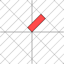
We see now that this new grid is transformed in the same way that the original grid was transformed by the diagonal matrix: the grid is stretched by a factor of 3 in one direction.
Now let’s use some definitions. M is a diagonal matrix (the entries outside the main diagonal are all zero) and both M and M’ are symmetric (if we get the columns and use them as new rows, we will get the same matrix).
Multiplying by a diagonal matrix results in a scaling effect (a linear transformation that enlarges or shrinks objects by a scale factor).
The effect we saw (the same result for both M and M’) is a very special situation that results from the fact that the matrix M’ is symmetric. If we have a symmetric 2 x 2 matrix, it turns out that we may always rotate the grid in the domain so that the matrix acts by stretching and perhaps reflecting in the two directions. In other words, symmetric matrices behave like diagonal matrices. — David Austin
“This is the geometric essence of the singular value decomposition for 2 x 2 matrices: for any 2 x 2 matrix, we may find an orthogonal grid that is transformed into another orthogonal grid.” — David Austin
We will express this fact using vectors: with an appropriate choice of orthogonal unit vectors v1 and v2, the vectors Mv1 and Mv2 are orthogonal.
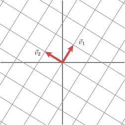
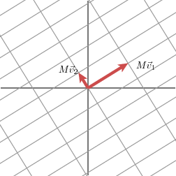
We will use n1 and n2 to denote unit vectors in the direction of Mv1 and Mv2. The lengths of Mv1 and Mv2 — denoted by σ1 and σ2 — describe the amount that the grid is stretched in those particular directions.
Now that we have a geometric essence, let’s go back to the formula:
M = UDV*
- U is a matrix whose columns are the vectors n1 and n2 (unit vectors of the ‘new’ grid, in the direction of v1 and v2)
- D is a diagonal matrix whose entries are σ1 and σ2 (the length of each vector)
- V* is a matrix whose columns are v1 and v2 (vectors of the ‘old’ grid)
Now that we understand a little about how SVD works, let’s see how LSI makes use of the technique to group texts. As Ian Soboroff shows on his Information Retrieval course slides:
- U is a matrix for transforming new documents
- D is the diagonal matrix that gives relative importance of dimensions (we will talk more about these dimensions in a minute)
- V* is a representation of M in k dimensions
To see how this works we will use document titles from two domains (Human Computer Interaction and Graph Theory). These examples are from the paper An Introduction to Latent Semantic Analysis.
c1: Human machine interface for ABC computer applications c2: A survey of user opinion of computer system response time c3: System and human system engineering testing of EPS
m1: The generation of random, binary, ordered trees m2: The intersection graph of paths in trees m3: Graph minors: A survey
The first step is to create a matrix with the number of times each term appears:
| termo | c1 | c2 | c3 | m1 | m2 | m3 | |-----------|----|----|----|----|----|----|| human | 1 | 0 | 1 | 0 | 0 | 0 || interface | 1 | 0 | 0 | 0 | 0 | 0 | | computer | 1 | 1 | 0 | 0 | 0 | 0 | | user | 0 | 1 | 0 | 0 | 0 | 0 | | system | 0 | 1 | 2 | 0 | 0 | 0 | | survey | 0 | 1 | 0 | 0 | 0 | 1 | | trees | 0 | 0 | 0 | 1 | 1 | 0 | | graph | 0 | 0 | 0 | 0 | 1 | 1 | | minors | 0 | 0 | 0 | 0 | 0 | 1 |
Decomposing the matrix we have this (you can use this online tool to apply the SVD):
# U Matrix (to transform new documents)
-0.386 0.222 -0.096 -0.458 0.357 -0.105-0.119 0.055 -0.434 -0.379 0.156 -0.040-0.345 -0.062 -0.615 -0.089 -0.264 0.135-0.226 -0.117 -0.181 0.290 -0.420 0.175-0.760 0.218 0.493 0.133 -0.018 0.044-0.284 -0.498 -0.176 0.374 0.033 -0.311-0.013 -0.321 0.289 -0.571 -0.582 -0.386-0.069 -0.621 0.185 -0.252 0.236 0.675-0.057 -0.382 0.005 0.085 0.453 -0.485
Matrix that gives relative importance of dimensions:
# D Matrix (relative importance of dimensions)
2.672 0.000 0.000 0.000 0.000 0.0000.000 1.983 0.000 0.000 0.000 0.0000.000 0.000 1.625 0.000 0.000 0.0000.000 0.000 0.000 1.563 0.000 0.0000.000 0.000 0.000 0.000 1.263 0.0000.000 0.000 0.000 0.000 0.000 0.499
Representation of M in k dimensions (in this case, we have k documents):
# V* Matrix (representation of M in k dimensions)
-0.318 -0.604 -0.713 -0.005 -0.031 -0.153 0.108 -0.231 0.332 -0.162 -0.475 -0.757-0.705 -0.294 0.548 0.178 0.291 0.009-0.593 0.453 -0.122 -0.365 -0.527 0.132 0.197 -0.531 0.254 -0.461 -0.274 0.572-0.020 0.087 -0.033 -0.772 0.580 -0.242
Okay, we have the matrices. But now the matrix is not 2 x 2. Do we really need the amount of dimensions that this term-document matrix has? Are all dimensions important features for each term and each document?
Let’s go back to the example of David Austin. Let’s say now we have M’’:
M'' = | 1 1 | | 2 2 |
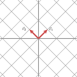
Now M’’ is no longer a symmetric matrix. For this matrix, the value of σ2 is zero. On the grid, the result of the multiplication is:
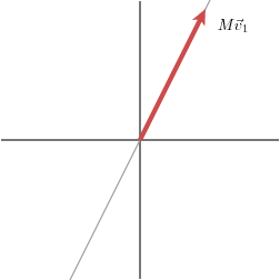
We have that if a value from the main diagonal of D is zero this term does not appear in the decomposition of M.
In this way, we see that the rank of M, which is the dimension of the image of the linear transformation, is equal to the number of non-zero values. — David Austin
What LSI does is to change the dimensionality of the terms.
In the original matrix terms are k-dimensional (k is the number of documents). The new space has lower dimensionality, so the dimensions are now groups of terms that tend to co-occur in the same documents. — Ian Soboroff
Now we can go back to the example. Let’s create a space with two dimensions. For this we will use only two values of the diagonal matrix D:
# D2 Matrix
2.672 0.000 0.000 0.000 0.000 0.0000.000 1.983 0.000 0.000 0.000 0.0000.000 0.000 0.000 0.000 0.000 0.0000.000 0.000 0.000 0.000 0.000 0.0000.000 0.000 0.000 0.000 0.000 0.0000.000 0.000 0.000 0.000 0.000 0.000
As Alex Thomo explains in this tutorial, terms are represented by the row vectors of U2 x D2 (U2 is U with only 2 dimensions) and documents are represented by the column vectors of D2 x V2* (V2* is V* with only 2 dimensions). We multiply by D2 because D is the diagonal matrix that gives relative importance of dimensions, remember?
Then we calculate the coordinates of each term and each document through these multiplications. The result is:
human = (-1.031, 0.440)interface = (-0.318, 0.109)computer = (-0.922, -0.123)user = (-0.604, -0.232)system = (-2.031, -0.232) survey = (-0.759, -0.988)trees = (-0.035, -0.637)graph = (-0.184, -1.231) minors = (-0.152, -0.758)
c1 = (-0.850, 0.214)c2 = (-1.614, -0.458)c3 = (-1.905, 0.658)m1 = (-0.013, -0.321)m2 = (-0.083, -0.942)m3 = (-0.409, -1.501)
Using matplotlib to visualize this, we have:
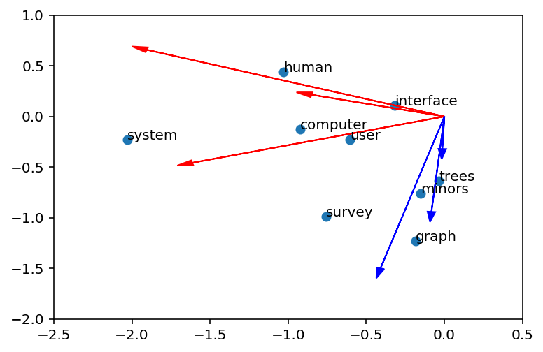
Cool, right? The vectors in red are Human Computer Interaction documents and the blue ones are of Graph Theory documents.
What about the choice of the number of dimensions?
The number of dimensions retained in LSI is an empirical issue. Because the underlying principle is that the original data should not be perfectly regenerated but, rather, an optimal dimensionality should be found that will cause correct induction of underlying relations, the customary factor-analytic approach of choosing a dimensionality that most parsimoniously represent the true variance of the original data is not appropriate. — Source
The measure of similarity computed in the reduced dimensional space is usually, but not always, the cosine between vectors.
And now we can go back to the dataset with theses from the Universities. I used the lsi model from gensim. I did not find many differences between the works of the Universities (all seemed to belong to the same cluster). The topic that most differentiated the works of the Universities was this one:
y topic:[('object', 0.29383227033104375), ('software', -0.22197520420133632), ('algorithm', 0.20537550622495102), ('robot', 0.18498675015157251), ('model', -0.17565360130127983), ('project', -0.164945961528315), ('busines', -0.15603883815175643), ('management', -0.15160458583774569), ('process', -0.13630070297362168), ('visual', 0.12762128292042879)]
Visually we have:
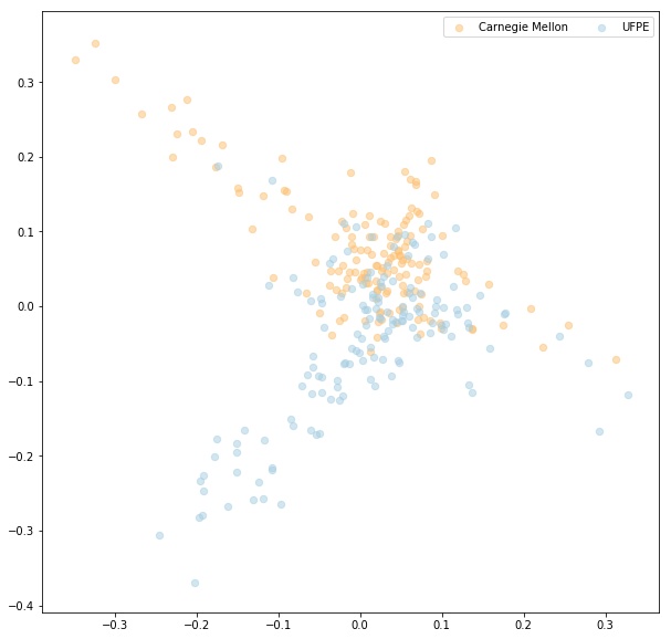
In the image the y topic is on the y-axis. We can see that Carnegie Mellon theses are more associated with ‘object’, ‘robot’, and ‘algorithm’ and the theses from UFPE are more associated with ‘software’, ‘project’, and ‘business’.
You can see the Jupyter notebook with the code here.
Step 2 — Investigating the nature of the works
I always had the impression that in Brazil, students produce many theses with literature review, while in the other Universities they made few theses like this. To check, I analyzed the titles of the theses.
Usually when a thesis is a literature review the word ‘study’ appears in the title. I then took all the titles of all the theses and checked the words that appear the most, for each University. The results were:


You can see the Jupyter notebook with the code here.
Findings
The sense I got from this simple analysis was that the themes of the works did not differ much. But it was possible to visualize what seems to be the specialties of each institution. The Federal University of Pernambuco produces more work related to projects and business and Carnegie Mellon produces more work related to robots and algorithms. In my view, this difference of specialties is not something bad, it simply shows that each university is specialized in certain areas.
A takeaway was that in Brazil we need to produce different works instead of just doing literature review.
Something important that I realized while doing the analysis (and that did not come from the findings of the analysis itself), was that only having the best thesis is not enough. I started the analysis trying to identify why they produce better works than us and what can we do to get there and become more well known. But I felt that maybe one way to get there is simply to show more of our work and to exchange more knowledge with them. The reason is because this can force us to produce more relevant articles and improve with feedback.
I also think that this is for everyone, both for university students and for us professionals alike. This quote that sums it up well:
“It’s not enough to be good. In order to be found, you have to be findable.” — Austin Kleon
And that’s it, thank you for reading!
If you found this article helpful, it would mean a lot if you click the ? and share with friends. Follow me for more articles about Data Science and Machine Learning.
Subscribe to my newsletter
Read articles from freeCodeCamp directly inside your inbox. Subscribe to the newsletter, and don't miss out.
Written by

freeCodeCamp
freeCodeCamp
Learn to code. Build projects. Earn certifications—All for free.